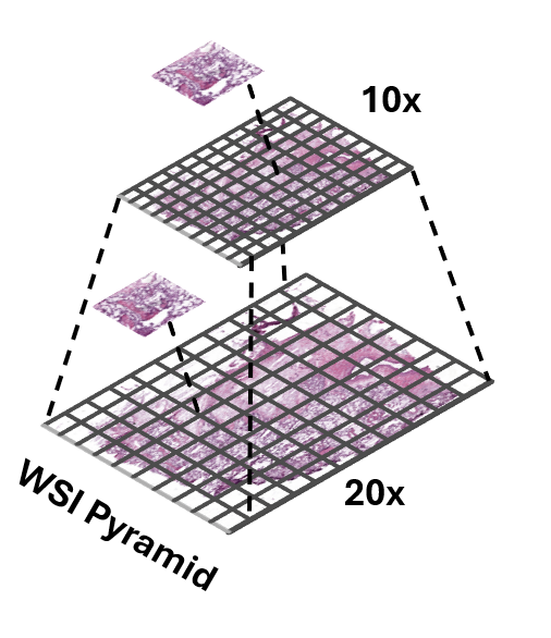
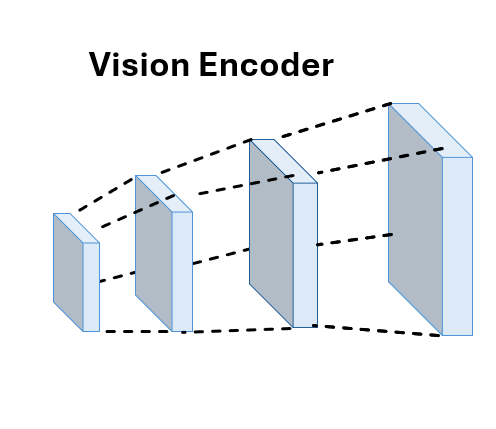
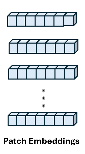
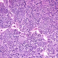
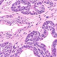
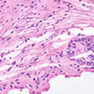
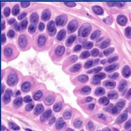
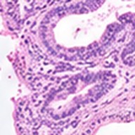
I single-handedly engineered the end-to-end pipeline, from raw slides to extracted features, on Marquette University’s GPU cluster.
Data processed
200+ TB
Whole-slide image (WSI) datasets
47
Patch-level datasets
20
Foundation models
25+
Magnification scales
3
NVIDIA V100 GPUs
48
TRIDENT contributions
7 pull requests submitted
I implemented patch encoder integrations for TRIDENT, the Mahmood Lab’s toolkit for large-scale whole-slide image processing.
NSF ACCESS allocation
CIS261298Awarded
Systematic evaluation of prompt-guided vision-language models for digital pathology
Awarded10,249 GPU hours on NCSA Delta for 2026, as the lead on the request.
ScopeBenchmark pathology foundation and vision-language models on 8 public datasets: more than 17,000 whole-slide images across cancer types.
QuestionsEncoder architecture, prompt sensitivity and automated prompts, token pruning, reasoning strategies and interpretability.
WorkflowTRIDENT segmentation and multi-resolution patching, reusable embeddings from several foundation models, then large-scale prompt-guided inference; about 35 TB of storage.
Expert-Guided Vision–Language Reasoning for Few-Shot Cancer Subtyping in Whole-Slide Pathology
Big ideaUse domain-specific expert roles and model-generated reasoning to guide few-shot cancer subtyping from whole-slide images.
MethodCombine four expert-role prompts and reasoning-informed text embeddings with 10×/20× visual features using learned patch prototypes and cross-attention.
FindingUnder the 16-shot, five-fold protocol, the best configurations reach AUC 0.9604 ± 0.0088 on TCGA-RCC and 0.8770 ± 0.0195 on TCGA-NSCLC, outperforming 20 MIL baselines.
ImpactExpert-derived language and multi-scale visual evidence can support subtyping with few labelled slides; gains depend on the encoder and prompting configuration.
TME-Context
ConferenceUnder review
Conditioning pathology vision–language models on quantitative tumor-microenvironment measurements
Big ideaGive pathology vision–language MIL models explicit tumor-microenvironment context: quantitative TME measurements derived from the H&E slide itself.
TC-LRAn H&E TME atlas model produces OpenTME measurements; after scaling, a regularized logistic regressor predicts the subtype from TME features alone.
TC-FusionBlends the native VLM prediction with the TME prediction: (1 − α)·pnative + α·pLR.
TC-AdapterGroups TME features into 16 phenotype tokens that cross-attend to the frozen VLM’s patch features, yielding TME-conditioned queries for the aggregator. Works with ViLa-MIL, MGPATH, FOCUS, MUSE, DyKo and MSCPT.
INVEX
Label-free FM ranking
Label-free pathology foundation model ranking via invariance and expressiveness
Big ideaRank pathology foundation models intrinsically, from their embeddings alone: no labels, no fine-tuning.
InvarianceA patch rotated by 90°, 180° or 270° has the same morphology, so its embeddings should stay close.
ExpressivenessEffective rank of the embeddings checks that different tissues stay apart instead of collapsing together.
Scale22 pathology FMs, 16 public patch-level benchmarks, 8+ organs and more than 1.2M patches.
Whole-slide image processing
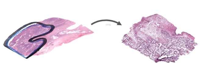
Tissue with pen marksAfter artifact filtering
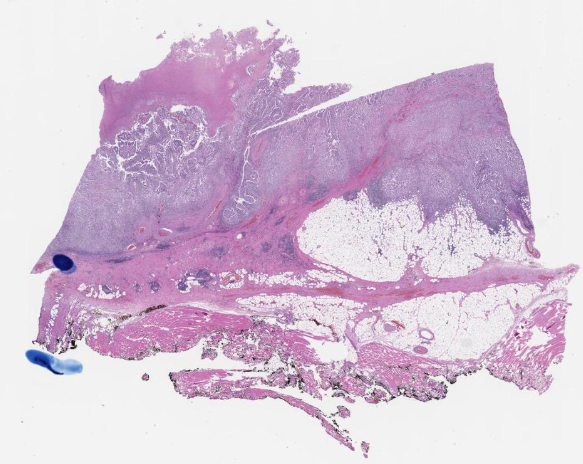
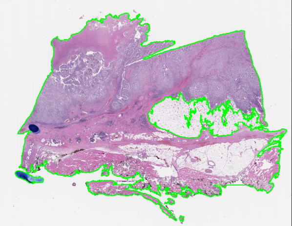
TRIDENT segments tissue, then applies GrandQC to exclude artifacts from the tissue mask. The retained contours are saved as GeoJSON for patch selection.
Why a queue?SimCLR’s negatives are limited to the batch. A queue of past keys holds far more.
Pseudocode
for x in loader: x_q, x_k = aug(x), aug(x)# f_k initialized from f_q q = f_q(x_q) # N x C k = f_k(x_k).detach()# queue: C x K keys, past batches l_pos = (q * k).sum(1, True) # N x 1 l_neg = q @ queue # N x K logits = cat([l_pos, l_neg], 1) labels = zeros(N) # positive at 0 loss = CE(logits / t, labels) loss.backward(); opt.step() # f_q f_k = m * f_k + (1 - m) * f_qenqueue(queue, k); dequeue(queue)# v2: MLP head, blur, cosine lr, t=0.2
Query and key views
crop, color jitter, flip, grayscale (v1)
Two random views of one patch; training pulls them together.
Two encoders
query encoder, trained by backpropagation
key encoder: no gradients, initialized from f_q
The key encoder is a slow, gradient-free copy of the query encoder.
Normalized embeddings
128ResNet-50, then fc to 128-d, ℓ2-normalized
detached; key batch shuffled across GPUs (shuffling BN)
Each view becomes a unit vector: or .
Dictionary as a queue
negatives come from the queue, decoupled from the batch size (256)
The dictionary of negatives can be far bigger than the batch.
InfoNCE over keys
the key of the same image, at index 0
0.07 in v1
Train to find its own key among .
Momentum update
momentum coefficient, 0.999
Slow drift keeps old and new keys in the queue comparable.
Update the queue
queuekeys from recent batches by a slowly changing encoder
This batch’s keys join; the oldest batch leaves.
MoCo v2 changes
Component
MoCo v1
MoCo v2
Projection head
Single linear layer
2-layer MLP with ReLU
Data augmentation
Standard augmentation
Stronger augmentation, including Gaussian blur
Learning-rate schedule
Step decay
Cosine decay
Temperature
0.07
0.2
Barlow Twins
H&E patch (unlabeled)
Two random augmentations(as in BYOL, incl. solarization)
View
random crop, then augment
View
random crop, then augment
Twin AEncoder ResNet-50Projector, 3 layers
Twin B, same weightsEncoder ResNet-50Projector, 3 layers
Shared weights
8,192-d embedding
8,192-d embedding
Cross-correlation of the two embeddingscomputed over the batch; 8 of the 8,192 dimensions shown
batch × , each column standardized
,
Diagonal → 1: each dimension is invariant to the augmentations
Off-diagonal → 0: dimensions carry non-redundant information
Training drives toward the identity
No negatives, predictor, stop-gradient or momentum encoder
Downstream: keep and its 2,048-d output ; drop
Pseudocode
# x: N unlabeled H&E patchesfor x in loader: y_a, y_b = augment(x), augment(x) h_a, h_b = f(y_a), f(y_b) # shared z_a, z_b = g(h_a), g(h_b) # N x D z_a = (z_a - z_a.mean(0)) / z_a.std(0) z_b = (z_b - z_b.mean(0)) / z_b.std(0) c = z_a.T @ z_b / N # D x D on = ((diag(c) - 1) ** 2).sum() off = (off_diagonal(c) ** 2).sum() loss = on + lambd * off loss.backward(); opt.step()# after training: keep f, use h
Two augmented views
crop, flip, color jitter, grayscale, blur, solarization
independent draws; blur and solarization odds differ per view
One encoder, shared weights
encoder (ResNet-50), the same weights for both views
2,048-d representation kept for downstream tasks
A wide projector
projector: 3 linear layers of 8,192 units
BN, ReLUafter the first two layers
Standardize each dimension over the batch
mean and standard deviation of dimension over the batch
a sample in the batch (2,048 in the paper)
Cross-correlation between the views
, entries between −1 and 1
embedding dimensions, not samples
Barlow Twins loss
5 × 10⁻³, weights the redundancy term
invariance: each dimension agrees across views
redundancy reduction: dimensions decorrelate
Target
identity matrix
nonegatives, predictor, stop-gradient or momentum encoder
VICReg
H&E patch (unlabeled)
Two random augmentations(as in BYOL, incl. solarization)
View
random crop, then augment
View
random crop, then augment
BranchEncoder ResNet-50Expander, 3 layers
Branch′Encoder ResNet-50Expander, 3 layers
Shared weights(or not: may differ)
8,192-d, not normalized
Invariance
Pull the two embeddings together (MSE)
VarianceKeep each dimension’s std above , per branchCovariance
Decorrelate dimensions within each branch
Component
What it does
Why
Invariance
Makes positive pairs similar
Learn augmentation-invariant representations
Variance
Ensures dimensions vary across images
Prevent collapse
Covariance
Reduces correlation between dimensions
Reduce redundancy
No negatives, stop-gradient, predictor or embedding normalization
Downstream: keep and its 2,048-d output ; drop
Pseudocode
for x in loader: x_a, x_b = augment(x), augment(x) y_a, y_b = f(x_a), f(x_b) z_a, z_b = h(y_a), h(y_b) # N x D sim = mse_loss(z_a, z_b); v = c = 0for z in (z_a, z_b): # each branch std = sqrt(z.var(0) + 1e-4) v += relu(1 - std).mean()for z in (z_a, z_b): C = cov(z) # D x D c += off_diag(C).pow(2).sum() / D loss = 25 * sim + 25 * v + 1 * c loss.backward(); opt.step()
Two augmented views
the image; and are its two views
crop, flip, color jitter, grayscale, blur, solarization
An encoder per branch
encoder (ResNet-50); its 2,048-d output is kept
usually equal to , but the branches may differ
Expander
expander: 3 layers of 8,192 units, discarded after training
a batch of embeddings, not normalized
Invariance
batch size (2,048 in the paper)
the only term that links the two branches
Invariance: Pulls two augmented views of the same image closer together.
Variance (hinge on the std)
target standard deviation, 1
10⁻⁴, keeps the square root stable
dimension across the batch, per branch
Variance: Prevents different images from all being mapped to the same representation.
Covariance, within each branch
covariance within one branch
vs. BarlowBarlow Twins correlates the two branches
Covariance: Encourages different embedding dimensions to carry nonredundant information.
Total loss
ImageNet defaults
nonegatives, stop-gradient, predictor or normalization
Invariance: Pulls two augmented views of the same image closer together.
Variance: Prevents different images from all being mapped to the same representation.
Covariance: Encourages different embedding dimensions to carry nonredundant information.
DINO
H&E patch (unlabeled)
Multi-crop augmentation(crop, color jitter, blur, …)
Student views (global + local crops)
2 global crops (high resolution)
•••
Several local crops (low resolution)
Global crops only(the student’s 2 global crops)
Teacher views (global only)
2 global crops (high resolution)
Student NetworkBackboneVision TransformerProjection head
Teacher NetworkBackboneVision TransformerProjection head
Cross-entropy between teacher and student output distributions from different views
Cross-entropy
EMA update
Pseudocode
# x: unlabeled H&E patchfor x in wsi_patches: crops = multi_crop(x) v_s = crops # 2 global + n local v_t = crops[:2] # same globals s = student(v_s)# teacher: stop gradientwith no_grad(): t = teacher(v_t) p_s = softmax(s / tau_s)# center, then sharpen p_t = softmax((t - c) / tau_t)# teacher global i vs student view j loss = mean(H(p_t[i], p_s[j])for i in (0, 1)for j in views if j != i) loss.backward() optimizer.step() # student teacher = ema(teacher, student) c = ema(c, t.mean(0))
Multi-crop views
all views of patch
2 global crops, 224 px
local crops, 96 px
number of local crops
Teacher views
the same 2 global crops
all views the student sees
Stop gradient
teacher weights, never trained by the loss
DINO loss
Student softmax
student logit for one view
output dimensions, 65,536 in DINO
student temperature, 0.1
Centered, sharpened teacher softmax
teacher logit
center, a running mean of
teacher temperature, warmed up from 0.04 to 0.07, below τₛ
Cross-entropy across views
cross-entropy
a teacher global crop; any other student view
EMA updates
student and teacher weights
momentum, 0.996 rising to 1
center momentum, 0.9 in the official code
batch mean of teacher outputs
MAE
H&E patch (unlabeled)
196 patches of 16 × 16 px
75% masked at random
25% visible
EncoderViT, visible patches only
Encoded tokens + shared mask token, with positions
Decoderlightweight
Masked patches predicted
Loss on masked patches onlymean squared error, per-patch normalized pixelspredictionvs.target
After pretraining, drop the decoder and run the encoder on all patches
Pseudocode
# x: N unlabeled H&E patchesfor x in loader: p = patchify(x) # B x 196 x 768 keep, mask = random_masking(0.75) z = encoder(p[keep] + pos[keep]) t = cat([z, m.repeat(n_masked)]) t = unshuffle(t) + pos p_hat = decoder(t)# p_hat: pixels for all 196 patches y = (p - p.mean(-1)) / p.std(-1) err = ((p_hat - y) ** 2).mean(-1) loss = err[mask].mean() loss.backward(); opt.step()# after: keep encoder, drop decoder
Patchify
one 16 × 16 px patch (7 × 7 of 196 shown)
Random masking
masked patches, sampled uniformly at random
Encoder on visible patches only
ViT encoder (ViT-B/16, L/16, H/14)
positional embedding of patch
25%of tokens enter the encoder, so pretraining is cheaper
Mask tokens join the sequence
one shared, learned mask token
Lightweight decoder
decoder: 8 blocks, 512-d, about 9% of ViT-L’s FLOPs per token
Reconstructed pixels
768= 16 × 16 × 3 pixel values per patch
Loss on masked patches
mean and std of patch i’s own pixels
the loss is computed on masked patches only
Downstream
discarded after pretraining
aug.random crop and flip only
iBOT
H&E patch (unlabeled)
Multi-crop + block masking(masks on the 2 global crops)
Student views (masked global + local crops)
2 global crops, 224 px (patches masked)
•••
Local crops, 96 px (no masks)
Global crops only(same 2 crops, no masks)
Teacher views (global only)
2 global crops, 224 px (unmasked)
Student NetworkBackboneViT, patch 16CLSpatchesShared head
Teacher NetworkBackboneViT, patch 16CLSpatchesShared head
Build one prototype per class by averaging molecular embeddings
Classify a slide by its nearest prototype, with no task-specific training
Tempus oFM
One patient’s record, grouped by dayclinical facts and molecular findings are text; H&E slides are images
Day 0DemographicsDay 14Diagnosis, stage, labsDay 21Biopsy: DNA, RNA, H&EDay 35Treatment startsDay 120ProgressionEmbed the patient here
Episode encoderGatorTron + FoNE
Episode token1,024-d, one per day
H&E slides
PRISM2frozen, 8,192-d
Projectorto 1,024-d
Token sequence up to
[CLS]day 0day 14day 21day 35day 120
+ modality embedding on every token
Time enters through rotary positions (RoPE)
Days with no data are skipped
Temporal encoder2 layers, bidirectional
Patient embedding, 1,024-d, from [CLS]
Pseudocode
# one patient, history up to t*days = group_by_day(facts)x_e = [episode_enc(d) for d in days]x_p = proj(prism2(slides)) # frozenseq = [cls] + tag(x_e, x_p)out = temporal_enc(seq, time=days)h = out[0] # 1024-d# h -> survival, benefit, subtypes
Episodes
episodeall facts attributed to one calendar day
dayscounted from the first observed event
Episode token
episode enc.finetuned GatorTron-base-2k, a clinical BERT
Pathology token
PRISM2frozen slide encoder; one embedding per biospecimen
Token sequence
learned modality embeddings
learned [CLS] token
empty daysleft out of the sequence
Temporal encoder
RoPErotary position encoding of relative time
attentionbidirectional over the whole history
Patient embedding
the day at which the patient is embedded
Scale
trained parameters
1,672,203patients in the development cohort
oFM: episode encoder
One day of factsillustrative patient
Diagnosis: lung adenocarcinoma, stage IV
ECOG performance status: 1
Hemoglobin: 11.2 g/dL
PD-L1 TPS: 45%
KRAS G12C, pathogenic
TMB-high
Serialized as textillustrative format; each number becomes [NUM]
diagnosis: lung adenocarcinoma
stage: IV
ecog: [NUM]
hemoglobin: [NUM] g/dL
pd-l1 tps: [NUM] %
kras: g12c pathogenic
tmb: high
Numbers keep their magnitudeFourier number embedding (FoNE)
Number losssmooth-L1 on the signed-log value at [NUM]
Because the decoder sees the day only through [CLS], that one vector has to hold everything. The decoder is discarded after pretraining; the encoder becomes the episode encoder.
Pseudocode
for ep in episodes: kept = drop_tokens(ep, p=0.6) cls = encoder(kept)[CLS] out = decoder(ep, cross=cls) l_tok = token_loss(out, ep) l_num = smooth_l1(num(out), u) loss = l_tok + l_num# then discard the decoder
Data
1,045,011patients used in Stage I
Corrupt the episode
drop probability; [CLS] and [SEP] are never dropped
Encode
must carry the whole day
Decode from [CLS]
decoderautoregressive; shares the encoder’s layers
cross-attnsees the encoder only through [CLS]
Token loss
rebuild every token of the uncorrupted episode
Number loss
read from decoder states at [NUM] positions
FoNEtrained jointly
Stage I objective
TSDAETransformer sequential denoising autoencoder
oFM: Stages II–III
Pick two anchor days on one patient’s timeline
[CLS]day 0day 14day 21day 35day 120
: an intervention (here, treatment start); : a later event (here, progression)
Student sees the days before ; teacher sees the days up to
Task: predict the patient’s state at
History before 70% of tokens masked
Studenttemporal encoder
History up to unmasked
EMA teacherno gradient
EMA,
PredictorFiLM residual MLP
Episode at + time gapwhat was done, and how far ahead
Latent prediction lossplus variance and covariance terms against collapse
now (t1)teacher (t2)prediction
Masked reconstruction
Masked tokens become a learned mask embedding
Heads rebuild the episode and pathology embeddings
Pathology tokens are also dropped with
Survival head
Input: history embedding + the episode at
Cox partial likelihood over the whole distributed batch
Two stages, one objective
II: encoders frozen; 386,382 treated patients (109,938 with H&E)
III: episode encoder unfrozen; 92,567 patients with DNA and RNA
MethodBenchmark 18 state-of-the-art vision and vision-language pathology encoders across 4,331 TCGA and CPTAC whole-slide images, evaluating similarity, representation alignment, and downstream transferability.
12
Patch Encoders
6
Slide Encoders
13
Downstream Tasks
4,331
Total Slides (TCGA & CPTAC)
47.5M+
Extracted Patches
3
Organs (Breast, Lung, Colon)
229
Property Tests
20x, 10x, 5x
Magnifications
Research questions
MOSAIC
Do independently trained pathology foundation models learn the same thing?
Central hypothesis: Independently trained pathology foundation models learn different coordinate systems over a shared underlying morphological manifold.
If that holds, representations should be alignable, semantic neighbourhoods should survive alignment, features should transfer between models, and a downstream classifier should be able to live inside one shared space.
Linear CKA
Do two encoders arrange the same patches the same way? Compare who sits near whom, ignoring rotation and scale.
Same patches, two encodersencoder Aencoder Brow i is the same patch in both
Center every featurethe mean (×) moves to the origin; only the shape is left
Sample-wise geometryn × n: how every pair of patches relates
Compare the two geometriesK⊙L→summed agreement10agreement
Invariances==same CKA score: only the arrangement of the patches matters
Pseudocode
X = enc_a(patches) # n x d_xY = enc_b(patches) # n x d_yX = X - X.mean(0)Y = Y - Y.mean(0)K, L = X @ X.T, Y @ Y.T # n x nhsic = norm(X.T @ Y) ** 2den = norm(X.T @ X) * norm(Y.T @ Y)cka = hsic / den# cka(X @ Q, 3 * Y) == cka(X, Y)
Two representations
the same patches, in the same row order
feature widths may differ
Run the same patches through two encoders.
Each patch is one row in and the same row in .
Center the features
centering matrix: removes each feature's mean
Subtract each feature’s average.
Now only the shape of the cloud matters, not where it sits.
Sample-wise geometry
how patch relates to patch in encoder A
For every pair of patches, measure how alike each encoder thinks they are.
Each encoder gets its own “who resembles whom” table.
Linear CKA
Frobenius norm, the square root of the sum of squared entries
1 means the two geometries match
Lay the two tables on top of each other and check agreement.
Normalize: 0 = unrelated, 1 = same geometry.
Invariances
notinvariant to an arbitrary invertible linear map
Rotating or uniformly rescaling an encoder changes nothing.
CKA compares structure, not the axes each model happened to pick.
Kernel CKA
Linear CKA with local, curved similarity: two encoders can match even if one bends the other’s geometry.
Curved, nonlinear structuresame two tissue types, bent differently
RBF kernel: local similaritynear patches score close to 1, far ones close to 0
Kernel matricespatches ordered along each curve: bands, not blocks
Center the kernels
Kernel CKA compares the centered kernels⊙Why a kernel helpsin kernel space a flat cut separates the curves0 · different geometry1 · same geometry
Pseudocode
X, Y = enc_a(patches), enc_b(patches)defrbf(A, s): D = cdist(A, A) ** 2 return exp(-D / (2 * s * s))K, L = rbf(X, s_x), rbf(Y, s_y)H = eye(n) - ones((n, n)) / nKc, Lc = H @ K @ H, H @ L @ Hnum = (Kc * Lc).sum()cka = num / (norm(Kc) * norm(Lc))
Nonlinear relationship
curveda straight-line comparison can miss this
Two encoders can bend the same structure differently.
A straight-line comparison may miss that they agree.
RBF kernel
bandwidth; often set from the median pairwise distance
Score each pair of patches by closeness: near ≈ 1, far ≈ 0.
σ sets how far “near” reaches.
Kernel matrices
one entry per pair of patches
Build one closeness table per encoder.
Neighbours along a curve light up a band near the diagonal.
Center the kernels
removes the mean similarity of every row and column
Subtract the average closeness of every row and column.
What is left: how much more or less alike a pair is than usual.
Kernel CKA
gives back linear CKA
Compare the two centered tables as in linear CKA.
Bent but matching geometries still score high.
SVCCA
Keep only each encoder’s dominant directions, then ask how well those directions can be lined up.
Two representationse.g. UNI-v2e.g. Prov-GigaPathsame n patches, different feature axes
SVD: keep 99% of the variance99%componentσ² (log)
CCA: most correlated directionsone weighted mix of features per encoder
Each new pair is uncorrelated with the earlier ones00.51…
mean
SVCCA scoreSame concept, different featuresdifferent encoders can encode one pattern with different features
Pseudocode
X, Y = enc_a(p), enc_b(p)defkeep99(A): U, s, _ = svd(A - A.mean(0)) r = cumsum(s**2) / sum(s**2) k = searchsorted(r, .99) + 1 return U[:, :k] * s[:k]Xr, Yr = keep99(X), keep99(Y)rho = cca(Xr, Yr) # canonical correlations# rho[0] >= rho[1] >= ... >= rho[K-1]svcca = rho.mean()
Two representations
the two encoders can have different widths
Two encoders, same patches, different numbers of features.
Do they capture the same information?
SVD: keep dominant directions
components kept per encoder
drops low-variance, noisy directions
Keep only the directions carrying 99% of each encoder’s variation.
This drops noisy, nearly empty directions.
CCA: first pair
weights: one linear combination of features per encoder
Find one mix of A’s features and one of B’s that move together most.
Their correlation ρ₁ says how well that best pair lines up.
More pairs
correlations come out in decreasing order
Find the next-best pair, unrelated to the ones already found.
Repeat: correlations come out from strongest to weakest.
SVCCA score
canonical pairs, at most min(k_a, k_b)
Average the correlations into one score.
High = the encoders share their dominant directions.
PWCCA
SVCCA where each matched direction counts by how much of the representation it actually carries.
Canonical directions of Xeach h is paired with a direction of Y
A plain mean weighs all equally1/K1/K1/K1/K1/K1/K1/K1/Kweak, noisy directionsthey count as much as the strong ones
How much of X each direction explainsΣsum each row, then normalize to 1
Each bar's width is its weight00.51width ∝ α
SVCCAPWCCA
PWCCA scorestrong directionsdominate the scorenoisy directionsbarely countweights from Xaverage both ways for symmetry
Pseudocode
rho, A, B = cca(X, Y)H = X @ A # canonical variates# SVCCA would use rho.mean()alpha = abs(H.T @ X).sum(1)alpha = alpha / alpha.sum()# wide bar: explains much of Xpwcca = (alpha * rho).sum()
Start from CCA
CCA weights, as in SVCCA
Start from the CCA directions and their correlations, as in SVCCA.
The problem with a plain mean
noiseweak, low-ρ directions count as much as strong ones
A plain average treats every direction the same.
Weak, noisy directions drag the score down unfairly.
Projection weights
feature of : one column
share of that direction accounts for
Ask how much of A’s features each direction actually explains.
Directions that carry more of the representation weigh more.
Weighted correlations
areabar width × height = contribution to the score
Each bar’s width is now its importance.
Important directions dominate; noise barely shows.
PWCCA score
asymmetricweights come from ; one can average both directions
The score is the importance-weighted average correlation.
Weights come from one side, so A→B and B→A can differ.
Procrustes similarity
Can one rigid rotation lay one point cloud on top of the other? The tighter the fit, the more similar.
Same patches, different orientationlines join the same patch
Center and normalise
Find the best rotation Rafter rotation the clouds overlap
Score: the nuclear norm of the cross-covariance
Stricter than CCACCA / SVCCAeach direction may be rescaled:the ellipse can match the circleProcrustesone rotation only:the ellipse never matches the circle
Pseudocode
X, Y = enc_a(p), enc_b(p)X = X - X.mean(0); X /= norm(X)Y = Y - Y.mean(0); Y /= norm(Y)U, s, Vt = svd(X.T @ Y)R = U @ Vt # orthogonalproc = s.sum() # nuclear normdist = 2 - 2 * proc # ||XR - Y||^2
Paired point clouds
pairsrow of and row of are the same patch
zero-pad the narrower one
Same patches, but the two clouds are rotated, scaled and shifted.
Center and normalise
removes global scale
Move both clouds to the origin and give them the same size.
Only the difference in orientation remains.
Best rotation
one rotation or reflection for the whole space
Find the single rotation that lays A’s cloud onto B’s.
Turning or mirroring only: no stretching.
Procrustes similarity
nuclear norm: the sum of singular values
Measure the overlap after that best rotation.
High = same shape up to a rigid turn.
A distance in disguise
stricterCCA may reweight each direction; Procrustes may not
CCA may stretch each direction to force a match; Procrustes may not.
So Procrustes is the stricter test of “same shape”.
Cosine RSA
Each encoder judges how alike every pair of patches is; RSA asks whether the two sets of judgements agree.
Each patch is a directioncolour = tissue class
Cosine similarity: the angleonly the angle counts,not the length
Similarity matricesred = same direction, blue = opposite
Keep the upper triangle and unroll itsame pairs, same order, in both vectors
Correlate the two patternsno alignmentcompares similarity patterns directlyangles onlyembedding lengths are ignoredSpearmanuses only the ranking of pairs
Pseudocode
X, Y = enc_a(p), enc_b(p)Xn = X / norm(X, axis=1, keepdims=True)Yn = Y / norm(Y, axis=1, keepdims=True)Cx, Cy = Xn @ Xn.T, Yn @ Yn.Tiu = triu_indices(n, k=1)vx, vy = Cx[iu], Cy[iu]rsa = spearmanr(vx, vy)[0] # or pearsonr
Embeddings as directions
patcheach one is a direction from the origin
Treat each patch’s embedding as an arrow from the origin.
Cosine similarity
angle between two embeddings; length is ignored
Compare two patches by the angle between their arrows.
Length is ignored; only direction counts.
Similarity matrices
RSMrepresentational similarity matrix
Fill a table with that similarity for every pair of patches.
One table per encoder.
Keep the upper triangle
the diagonal is always 1 and the matrix is symmetric
Keep each pair once and line the pairs up as a list.
Both encoders’ lists use the same pair order.
Correlate the patterns
Pearson, or Spearman to compare rankings only
Correlate the two lists.
High = the encoders agree on which patches are alike.
Distance correlation
Do distances in one encoder predict distances in the other? Catches any dependence, linear or not.
Pairwise distancesfrom every patch to every other, in X and in Y
Distance matricesbright = close, dark = far
Double centeringrow meanscolumn meansevery row and column now averages to zero
A = cdist(X, X) # n x nB = cdist(Y, Y)defdc(D): r, c = D.mean(1, keepdims=True), D.mean(0) return D - r - c + D.mean()Ah, Bh = dc(A), dc(B)dcov2 = (Ah * Bh).mean()dvar = sqrt((Ah**2).mean() * (Bh**2).mean())dcor = sqrt(dcov2 / dvar)
Pairwise distances
distanceswork for any widths d_x and d_y
Measure the distance between every pair of patches, in each encoder.
Distance matrices
one entry per pair of patches
Collect them into two distance tables.
Double centering
mean of row ; ā.. is the grand mean
Remove each row’s and column’s average distance.
This keeps how unusually close or far each pair is.
Distance covariance
double-centered the same way
Multiply the two tables entry by entry and average.
Large when both encoders flag the same pairs as unusual.
Distance correlation
Normalize to 0–1; it is 0 only if the two are independent.
Unlike ordinary correlation, it also catches curved links.
Metrics side by side
The seven similarity metrics: each ignores some changes and catches others. That is why they can disagree on the same pair of encoders.
Score unchanged by
Sees nonlinear relations
Watch out
Metric · what it compares
Rotation
Scale
Shift
Any linear map
Linear CKAWho sits near whom, as one Gram matrix
Dominated by the largest-variance directions
Kernel CKAThe same, with a local RBF closeness
The bandwidth σ changes the answer
SVCCAThe best-matched directions after SVD
Depends on how many directions you keep
PWCCACCA directions, weighted by importance
One-sided by design; averaged both ways
ProcrustesOverlap after one best rotation
Rigid only: a stretched copy scores lower
Cosine RSAAgreement of pairwise-similarity rankings
Ignores embedding length entirely
Distance correlationWhether distances co-vary, in any way
Memory grows with n², from n × n distance tables
The score ignores this change The score is sensitive to it
GCCA
Find one shared coordinate system that every encoder can be linearly mapped into.
Many encoders, same patchese.g. UNI-v2e.g. CONCHe.g. Virchow2
What each view can express++=patches every view agrees on add upn × n, one per encoder
The shared space Geigenvaluesdirections shared by all encoders
Map every view onto Geach encoder gets its ownlinear map W
One shared coordinate systemGX1X2X3star:every encoder talks to G onlylinear:one matrix W per encodernew patch:any encoder, same coordinates
Pseudocode
Xs = [enc(p) for enc in encoders]C = lambda X: inv(X.T @ X + eps * I)Ps = [X @ C(X) @ X.T for X in Xs]vals, vecs = eigh(sum(Ps))G = vecs[:, -k:] # n x kWs = [C(X) @ X.T @ G for X in Xs]Zs = [X @ W for X, W in zip(Xs, Ws)]# every Z_m is close to G
Many encoders
encoders; shared patches
Several encoders, the same patches, each with its own axes.
What each view can express
projects onto what view can express
small ridge for stability
Work out which patterns each encoder can express.
Add them up: patterns every encoder can express stand out.
The shared space
shared dimensions
The strongest shared patterns become the common space .
Map every view
a linear map per encoder
Give each encoder its own linear map into .
After mapping, all encoders’ points land on the same spots.
Objective
MAXVARthis formulation of GCCA
Everyone connects to one shared hub.
A new patch from any encoder gets the same coordinates.
MCCA
Find one projection per encoder so that all encoders agree with each other, pair by pair.
Many encoders, same patchese.g. UNI-v2e.g. CONCHe.g. Virchow2
Every pair is comparedX1X2X3no central reference: encoders agree with each other
One projection per encodersame patches, three 1-D summaries
Maximize the sum of pairwise correlationsall three scatter plots tighten at once
MCCA vs GCCAGCCA: starGX1X2X3MCCA: all pairsX1X2X3both are linear; GCCA fits a shared target G,MCCA makes the encoders agree with each other directly
Pseudocode
Xs = [enc(p) for enc in encoders]C = cov(hstack(Xs)) # blocks C_mlD = block_diag(C_11, ..., C_MM)# z_m = X_m @ w_mvals, W = eigh(C, D) # generalizedWs = split(W[:, -K:], dims)Zs = [X @ Wm for X, Wm in zip(Xs, Ws)]
Many encoders
encoders, same patches
Several encoders, the same patches.
Every pair
all pairsevery encoder is compared with every other
No shared hub: compare every pair of encoders directly.
One projection per view
weights: one linear combination per encoder
Squash each encoder’s features into one number per patch.
Sum of pairwise correlations
cross-covariance between views and
SUMCORthis sum-of-correlations criterion
Choose the squashing weights so every pair agrees as much as possible.
All pairwise scatter plots tighten at once.
More components
solvea generalized eigenproblem on the block covariance
GCCA aligns everyone to a shared target; MCCA aligns them to each other.
Both are linear.
Generalized Procrustes
Rotate every encoder onto a running average shape until they all settle on one consensus.
Center and normalise each viewe.g. UNI-v2e.g. CONCHe.g. Virchow2
Start from one view as the mean
Rotate every view onto the mean
Update the mean and repeatrotate↓average1234567iteration
Consensus shaperigid:rotations only, no stretchingconsensus:the mean shape of all encodersstrict:shapes must truly match
Pseudocode
Xs = [center_unit(X) for X in Xs]mean = Xs[0]for it in range(T): Rs = [procrustes(X, mean) for X in Xs] Al = [X @ R for X, R in zip(Xs, Rs)] mean = sum(Al) / M mean /= norm(mean)aligned = Al # one rotation per view
Center and normalise
zero-pad to a common width
Center each encoder’s cloud and give it unit size.
Pick a reference
referenceany view works; the result is the same up to one rotation
Take one encoder as the first guess of the average shape.
Rotate onto the mean
rotation or reflection only: shapes are kept
Rotate every encoder onto that average shape.
Rotation only: shapes are never stretched.
Update the mean, repeat
repeatuntil the mean stops moving
Average the rotated clouds into a new mean, then repeat.
The misfit shrinks until the mean stops moving.
Objective
the consensus shape all encoders share
Result: one consensus shape, plus one rotation per encoder.
Joint PCA
Put all encoders’ features side by side and keep the few directions that explain them together.
Views of different widthssame n patches (rows), different feature counts
Scale and concatenateeach block divided by its own norm first
PCA on the joint matrixσdirections of largest joint variance
Shared coordinates and per-view loadingsone row per patch,shared by all encodersloadings split by view
Xs = [enc(p) for enc in encoders]Xs = [X - X.mean(0) for X in Xs]Xs = [X / norm(X) for X in Xs]Xc = hstack(Xs)U, s, Vt = svd(Xc, full_matrices=0)Z = U[:, :k] * s[:k] # n x kVs = split(Vt[:k].T, cumsum(dims)[:-1])
Views
widths may differ
Each encoder gives a feature table of a different width.
Scale and concatenate
a common scaling so no view dominates
centered view
Scale each table so none dominates, then glue them side by side.
PCA on the joint matrix
joint principal directions
Run PCA on the glued table.
Keep the few directions that explain the most combined variation.
Shared coordinates
size of the shared subspace
Those directions give every patch a short shared coordinate.
Each encoder owns a slice of the directions.
Per-view loadings
rows of that belong to view
A patch’s coordinate is the sum of every encoder’s contribution.
No agreement goal: it chases variance, so scaling matters.
Shared autoencoder
Learn nonlinear maps into one small code from which every encoder’s features can be rebuilt.
Each encoder, its own featurese.g. UNI-v2e.g. CONCHe.g. Virchow2the same patch, three embeddings of different sizes
Nonlinear encoderseach MLP squeezes its view into k numbers
One shared bottleneckthe same patch gets the same code from any encoder
Decode every view from the code
Train: rebuild everything from anythingtraining stepslossnonlinear:can unbend curved geometrycross-rebuild:any code rebuilds every viewlearned:needs training, unlike the others
Pseudocode
xs = [enc(p) for enc in encoders]zs = [E[m](xs[m]) for m in range(M)]align = sum(mse(zs[m], zs[l]) for m < l)rec = sum(mse(D[l](z), xs[l]) for z in zs for l in range(M))loss = rec + lam * alignloss.backward(); opt.step()
Inputs
widths may differ
Each encoder describes the same patch with a different-length vector.
Encode
small MLP per encoder
bottleneck size
A small neural network per encoder squeezes it into a short code.
One shared bottleneck
same patchits codes should coincide
Train the codes from all encoders to agree for the same patch.
Decode every view
decoder for view
From that single code, rebuild every encoder’s features.
Training loss
weight on agreement; one common recipe, details vary
Training cuts rebuild error and disagreement together.
Being nonlinear, it can line up curved structure.
Aligners side by side
The five alignment methods all build one shared space from many encoders. They differ in what they treat as the reference and how freely each encoder may move.
Method
Shared reference
Map for each encoder
Objective
Watch out
GGCCA
One central space G
A linear map W per encoder
Every encoder agrees with G
Linear only
MCCA
None: encoders meet pairwise
A linear projection per encoder
Sum of all pairwise correlations
Pairs grow fast as encoders are added
Generalized Procrustes
A consensus mean shape
A rotation per encoder
Least-squares fit to the mean
Cannot stretch; pad to one width
Joint PCA
Top joint principal axes
PCA loadings, split by encoder
Most joint variance
Variance, not agreement; scaling matters
Shared autoencoder
One small shared code
An MLP encoder and decoder per encoder
Rebuild every view; codes agree
Needs training and tuning
Icons, with example encoders: UNI-v2 CONCH Virchow2
Cross-model transfer
Encode a patch with one model and decode it as another: can a model built on B use A’s features unchanged?
Paired patches on one grid10× · 256 pxfittestrows pair up only when crops are identical
Encode with model Acenter · scale · mapshared space
Decode as model Bor decode back to A: the round-trip ceiling
Three tests, each harder1 · Fidelityclose to B’s real vector?2 · Retrievalown patch ranked first?3 · Linear probeB’s classifier still right?≈query#1 same patch#2#3#4#5recall@k in B’s own space● real B △ translated from A
Every ordered pair, against its ceilingAABBCCDDtargetsourcediagonalround trip: the cost of the shared space aloneoff-diagonalthe extra cost of crossing modelsA→B vs B→Atransfer is directional
same gridsame magnification and patch size, so rows pair up
Use patches cut identically for both encoders, so rows line up.
Fit on 70% of patches; test on the other 30%.
Encode with model A
center, scale, then the aligner’s map; GCCA by default
shared size, 64 by default
Map encoder A’s embedding into the shared space.
Decode as model B
back out of the shared space, into B’s own features
Decode that code as if encoder B had produced it.
Decoding back into A instead gives the best-case round trip.
Three tests, each harder
probetrained only on B’s real embeddings
Is it close to B’s real vector?
Does it find its own patch in B’s index?
Does a classifier trained on real B still get it right?
Against the round trip
directionalA → B and B → A can differ
Score every ordered pair of encoders.
The gap to the round trip is the true cost of switching models.
Layer-wise alignment
Compare every block of one model with every block of another: where do they agree, and where do they part?
Hook every blockmodel Amodel Ba forward hook after each transformer block
One vector per blockCLSpatch tokensCLS tokenmean of tokensdefault: CLS · CNN maps: global average
Every block against every blockinoutblocks of B →blocks of A →bright diagonal:they progress togetherridge fades late:they part waysillustrative pattern
Best match for each block of Arelative depth of ACKAbest matchsame relative depth
Where do they part ways?earlylatedivergencedivergence depthstays below τ after thisearly − late> 0: early layers shareddepth offsetwho gets there first
same tissuepatches re-cropped at the recorded coordinates
vision toweronly CONCH’s and MUSK’s image encoders are hooked
Run the same patches through both models.
Record what every layer produces, not just the final output.
One vector per block
CNNfeature maps are global-average pooled
Squash each layer’s tokens into one vector per patch.
Block-to-block CKA
every block against every block, on the same patches
Compare every layer of A with every layer of B using CKA.
Alignment trajectory
B reaches that representation earlier than A
For each layer of A, find the most similar layer of B.
Tracing the matches shows whether they progress in step.
Where they part ways
divergence threshold, 0.5 by default; report it
Find where the best match drops below a threshold for good.
Shared early, different late: the models diverge with depth.
SEAL: paired spots and patches
Towards Spatial Transcriptomics-driven Pathology Foundation ModelsHemker, Song et al., Mahmood Lab, arXiv 2026Paper ↗Code ↗Hugging Face ↗
A Visium sectionspots on a hexagonal gridone spot55 µm
224 px patch, three scales1.0 µm/px0.5 µm/px0.25 µm/pxone picked at random for each spot
Neighbour smoothingcentre spotmean of up to 6 neighbours
Expression vector for the spotraw countsnormalisedkeep variablegenes
MAPLE-TrainHEST-1k public studies + Mass General Brigham data723,250spot–patch pairs353samples14organstrain 80%val 10%test 10%split by patient, stratified by organ
Pseudocode
for spot in visium_sample.spots: s = random.choice([0.25, 0.5, 1.0]) x = crop(wsi, spot.center, 224, mpp=s) c = spot.counts g = log1p(1e4 * c / c.sum())[hvg] g = (g + G[spot.nbrs].mean(0)) / 2 pairs.append((x, g)) # 723,250 pairs
Paired measurements
Visiumspatial transcriptomics: expression measured in 55 µm spots on a hexagonal grid
Image side
spot centroid
one magnification sampled per spot, per step
Gene side
highly variable genes (Seurat v3)
2,000genes in training
Spatial smoothing
up to 6 neighbours on the hexagonal lattice
Training set
723,250 pairs from 353 samples, 14 organs
split80/10/10 by patient, stratified by organ
SEAL: two encoders
Five pathology FMs, one recipeCONCHLoRA in last 3H0-miniLoRA in last 3Phikon-v2LoRA in last 7UNI-v2-hLoRA in last 5Virchow-v2LoRA in last 7
Vision encoder: frozen weights + LoRApatchblock 1block 2block 3block 4block 5block 6block 7block 8block 9block 10block 11block 12LoRAinside one attention projection+r = 8: only the orange matrices train
Omics encoder: a VAELinear · BN · ReLU
Planar flows reshape the latent density
mirrored decoderthe gene latent matches the image embedding size, so Stage II can compare them
Pseudocode
vit = load_fm("uni_v2") # any of 5vit.requires_grad_(False)add_lora(vit.blocks[-k:], r=8, alpha=8)e = mlp(g) # Linear-BN-ReLUmu, logvar = w_mu(e), w_var(e)z = mu + exp(logvar / 2) * randn_like(mu)for f in planar_flows: z = f(z)g_hat = decoder(z) # mirrored MLPassert z.shape[-1] == vit.embed_dim
LoRA rank and scale, attention layers of the last blocks
Omics: a VAE
MLP features: linear, batch norm, ReLU
sampling noise
Planar flows
learned flow parameters; each step bends the latent density
Shared size
512 · 1,536 · 1,024 · 1,536 · 2,560 for the five backbones
SEAL Stage I: gene warm-up
Batch
Gene VAEencode · decode
Recon.
Per-gene error
Correlationevery pair of genes(true vs. reconstructed)
invarianceredundancy
Why warm up firstThe gene encoder starts from scratch while thevision encoder is a strong pretrained FM.Training it alone first gives Stage II a geneembedding worth aligning to.batchepochslearning ratecosineschedule
Pseudocode
g = batch.genes # B x Gg_hat, kl = vae(g)l_mse = ((g - g_hat) ** 2).mean()C = xcorr(g, g_hat) # G x G, over batchl_rec = l0 * ((1 - C.diag()) ** 2).sum() + l1 * (C.offdiag() ** 2).sum() + l2 * l_mse + klopt = Adam(vae.parameters(), lr=5e-4)
A batch of spots
batch of spots; each row is one expression vector
Encode and decode
VAE reconstruction
Per-gene error
number of genes
Gene–gene correlation
index over the batch
matrix, Barlow-Twins style
Diagonal up, off-diagonal down
redundancy weighted below invariance
Schedule
384batch size; up to 3 epochs, lr 5·10⁻⁴, cosine schedule
Genes from the imagethe gene decoder reads the image embedding
Forget which studyGRLstudy Astudy Bstudy Creversed gradient
One objective, four termscontrastive+genes from image+gene reconstruction+domain-adversarialTrainable: LoRA adapters, gene VAE, decoder and heads. The FM weights never change.
From raw channels to a training samplequality controlbad stains and artefacts dropped
z-scoreDAPICD3CD8
one training image: DAPI + 2 random markersDAPIpanCKCD20224 crop · flips · 90° rotationssubset drawn from 23 tissue × platform groups
Pseudocode
X = load_multiplex(roi) # H x W x M# 30 sources, 8 platforms, 16 tissuestiles = tile(X, 256, overlap=0.5)tiles = [t for t in tiles iftissue_ok(t)]t = (t - mu[markers]) / sd[markers]sub = random.choice(subsets) # 23x = t[[dapi, *sample(panel, 2)]]
A multiplex image
tens of markers per section (up to ~50–60)
channelone antibody, one fluorescence image
SPM-47M sources
30sources: 56% public, 44% in-house
8fluorescence platforms, e.g. CODEX, MxIF, COMET, IBEX
Patches
px patches, 50% overlap
single-marker patches from 3.67M multiplex patches
Quality control
QCmarkers checked against vendor / Human Protein Atlas staining; tissue mask drops folds, blur, saturation
Per-marker normalisation
per-marker statistics over the whole corpus
Training sample
23tissue–technology subsets; pick one, then a patch
aug224 crops, flips, 90° rotations
KRONOS: a marker-aware ViT
Each marker tokenised on its ownDAPICD3panCKshared weights
Marker codefixed sinusoidsdimension
Adding the codes++=
One sequenceN locations × M markersCLSDAPI tokensCD3 tokenspanCK tokens12 transformer blocks · self-attention across locations and markers
Three kinds of outputimagethe CLS token: one vector per imagemarkermean over locations, one per markertokenmarkers concatenated at each location
Pseudocode
for j in markers: xb[j] = embed(x[j]) # sharedm = sincos(marker_ids, D) # fixedz = xb + m[:, None] + pos[None]z = vit_blocks(cat([cls, z.flatten(0, 1)]))img = z[0]marker = z[1:].view(M, N, D).mean(1)tokens = z[1:].view(M, N, D)
Tokenise each marker
16 × 16 px patch of marker
same weights for every marker
Marker identity
fixed, not learned: an unseen marker just takes an unused index
Add the codes
Visual embedding of spatial patch from protein marker
Marker identity code: which protein?
Spatial positional embedding: where in the tissue patch?
Final token given to the transformer
For the CD3 channel, KRONOS constructs:
One sequence
tokens: attention mixes locations and markers
ViT-S/16backbone
Three outputs
image-level output
GigaTIME: paired H&E and mIF
Multimodal AI generates virtual population for tumor microenvironment modelingMicrosoft Research, Providence and UW, CellPaper ↗Code ↗Hugging Face ↗
Same tissue, two stainsH&E whole slide≈100k × 100k pxCOMET mIF of one region≈40k × 40k px, 21 proteins
Registration (VALIS)mIF warped onto the H&E
Keep well-aligned tilesH&E cellsmIF nuclei0.2StarDist on both, thendrop tiles that fail
40Mpaired cells21protein channelsCOMETmIF platform256²px training tiles
Pseudocode
he, mif = load(case) # H&E WSI, COMET mIFmif = valis_register(mif, he)A, B = stardist(he), stardist(mif.dapi)keep tiles if dice(A, B) >= 0.2Y = mif > thresholds # per channelpairs.append((he_tile, Y)) # 256 x 256
Same tissue, two stains
COMETsequential mIF platform; same tissue as the H&E slide
Registration
rigid + non-rigid warp found by VALIS
image dissimilarity
Quality filter
StarDist cells on H&E / on mIF DAPI; 0.2 set from 100 hand-labelled pairs
Per-pixel targets
CD8 intensity
1280100451101402026090805203
t = 50 example
binary map
0110011001100000
Training pairs
2321 proteins + 2 background channels
cells in the paired training data
GigaTIME: a UNet++ translator
UNet++H&E 256²encoder
dense skip connections
23 maps, 256²
BCE + Dicepredictiontargetevery pixeloverlap, robust to rare markers
Training300epochsAdamlr 10⁻³32batchCNNUNet++settings from the released training command
Pseudocode
x = he_tile # 3 x 256 x 256X[i][0] = conv(down(X[i-1][0]))X[i][j] = conv(cat(X[i][:j], up(X[i+1][j-1])))# every node sees all earlier nodes in its rowY_hat = sigmoid(conv1x1(X[0][4])) # 23 mapsloss = bce(Y_hat, Y) + 1 - dice(Y_hat, Y)# 300 epochs, Adam 1e-3, batch 32
Encoder
encoder node at depth
downsampling
Nested decoders
upsampling from the node below
Dense skips
concatenation: dense skip connections across the row
Output head
2321 protein + 2 background channels
BCE + Dice
Diceoverlap per channel; helps sparse markers
Training
300epochs; Adam, lr 10⁻³, batch 32 (released recipe)
PyTorch pipeline: Dataset
__init__store what every sample will needself.data…self.labels02110…self.transformv2.Compose([…])Runs once, when the dataset is built.Keep it light: arrays or file paths,not every decoded image.
__len__how many samples there are12len(ds) = NThe DataLoader relies on N to:• count batches: ⌈N / B⌉ per epoch• shuffle: a permutation of range(N)• split: random_split(ds, [0.8, 0.2])
__getitem__return one sample and its labelds[7]y = 0x₇ passes through the transform:1. RandomResizedCrop2. HorizontalFlip3. ToDtype4. Normalize(x′, y)Called once per index, usuallyinside a DataLoader worker.
A sample can be any structureImage classification(x_k, y_k)image, labelObject detection(x_k, y_k, b_k)image, label, boxGraph learning(f_k, e_k, y_k)features, edges, label
PyTorch
class CustomDataset(Dataset): def __init__(self, data, labels, transform=None): self.data = data self.labels = labels self.transform = transform def __len__(self): return len(self.data) def __getitem__(self, index): x = self.data[index] y = self.labels[index] if self.transform: x = self.transform(x) return x, y# detection: return x, y, box# graphs: return feats, edges, y
__init__
dataan array in memory, or file paths read lazily
transforma v2.Compose pipeline, applied per sample
__len__
batch size
__getitem__
the transform: random for training, fixed for evaluation
Samplerdecides which indices, in what orderSequentialSampler012345same order every timeRandomSampler305142a shuffled order (shuffle=True)SubsetRandomSampler629random order within given indicesWeightedRandomSampler114101draws by weight, with replacementBatchSampler[0 1 2] [3 4 5]wraps a sampler: lists of indicesDistributedSamplerGPU0: 0 2 4 GPU1: 1 3 5one shard per GPU processimplement__iter__(__len__ optional)All subclass torch.utils.data.Sampler and yield indices, not data.
BatchSamplerdrop_last=False01234567894 batchesdrop_last=True01234567893 batches10 samples, batch_size=3: the last batch has 1 sample, or is dropped
Collator(, 0)(, 1)(, 1)collate011X [3, D]y [3]default_collate: adds a batch dimension, turns NumPy and numbersinto tensors, and keeps structure (a dict in gives a dict out).
Sampler, then batchesindices 0 … N−101234567891011shuffled order π, new every epoch72100511381946batch 1batch 2batch 3worker 0ds[7]ds[5]worker 1ds[10]ds[3]workers call ds[i] in parallel while the GPU trains
Collate into tensors0110X: [B, D]y: [B]collate_fn stacks the four samples
To the GPUCPU RAMpinnedGPU.to(device, non_blocking=True)
PyTorch
# 1. a Dataset: length + indexingclass PairDataset(Dataset): def __len__(self): return len(self.X) def __getitem__(self, i): x = self.tf(self.X[i]) # augment return x, self.y[i]dl = DataLoader(ds, shuffle=True, batch_size=4, num_workers=2, pin_memory=True)for X, y in dl: # collate_fn stacks X = X.to(device, non_blocking=True) y = y.to(device)
Dataset contract
__len__number of samples N
__getitem__loads sample i and applies the transform
transformnormalization, plus random augmentation for training only
Shuffle
a new random order each epoch
Mini-batches
batch size; N/B batches per epoch
Workers
num_workersseparate processes call ds[i]
prefetchnext batches load while the GPU computes
Collate
features per sample
number of classes
Host to device
pin_memorypage-locked RAM for fast copies
non_blockingcopy overlaps with compute
PyTorch pipeline: training
One batchX: [B, D]model.train()dropout on;batch-norm uses batch stats
Forward, then backwardLinear + ReLULinearlogits z[B, K]autocast bf16∇W₁∇W₂
Loss00.2210.6120.17softmax(z) for one sample, true class 1class−log 0.610.49CrossEntropyLoss averages over the batchloss.backward()
Clip, step, schedulegradients clipped, AdamW step, then the lr scheduleW₁W₂lrwarmup, then cosine decay
Repeatstepsloss
PyTorch
model = MLP().to(device)params = list(model.parameters())opt = AdamW(params)sched = cosine_with_warmup(opt)amp = torch.autocast("cuda", torch.bfloat16)loss_fn = nn.CrossEntropyLoss()for epoch in range(epochs): model.train() for X, y in dl: with amp: z = model(X) # forward loss = loss_fn(z, y) opt.zero_grad(set_to_none=True) loss.backward() # autogradclip_grad_norm_(params, max_norm) opt.step(); sched.step()# log loss, then validate
Training mode
train()turns on dropout and batch-norm updates
Xone batch from the DataLoader
Forward pass
all weights and biases
autocastruns matmuls in bfloat16: faster, less memory
Cross-entropy loss
classes
Backward pass
zero_gradclears last step’s gradients
backwardautograd fills .grad for every parameter
Clip, step, schedule
clip_grad_norm_caps the gradient norm so one bad batch cannot blow up
AdamWscales each step by running gradient statistics
schedulerwarms η up, then decays it over training
Iterations and epochs
stepone batch: forward, backward, update
epochone pass over all N samples
PyTorch pipeline: evaluation
model.eval()DropoutonoffBatchNormbatch statsrunning statssame weights, same answer every run
torch.no_grad()no graphno gradients kept: less memory, faster
Validation looptrue labels yargmax ŷ0211model0✓2✓1✓2✗0210model0✓2✓1✓0✓2102model1✗1✓0✓2✓val loader: shuffle=False, same order every epochaccuracy on these batches10 / 12
Train vs validationepochlossoverfittingtrain lossval lossbest.ptpatience: 3 epochsstopreload the best weights for testing:model.load_state_dict( torch.load("best.pt"))
PyTorch
@torch.no_grad()def evaluate(model, val_dl): model.eval()# no_grad: no graph, no .grad tot, hit, n = 0.0, 0, 0 for X, y in val_dl: X, y = X.to(device), y.to(device) z = model(X) tot += loss_fn(z, y).item() * len(y) hit += (z.argmax(1) == y).sum().item() n += len(y) return tot / n, hit / nfor epoch in range(epochs): train_one_epoch(model, dl) val_loss, val_acc = evaluate(model, val_dl) if val_loss < best: best, bad = val_loss, 0 torch.save(model.state_dict(), "best.pt") else: bad += 1 if bad == patience: break
Evaluation mode
eval()dropout off; batch-norm uses running mean and variance
train()switch back before the next epoch
No gradients
no_gradautograd records nothing inside it
inference_modea stricter, slightly faster variant
Validation pass
𝟙
shuffle=Falsesame order every epoch, so runs compare
lossweighted by batch size, so the last small batch counts fairly
batch statistics per channel; running averages in eval
learned scale and shift: 2 × 16 params; plus 32 running-stat buffers
ReLU and Dropout
drop probability
Max pooling
stridedefaults to the kernel size
Flatten
start_dim1 by default, so the batch stays separate
Linear
params4096 × 10 weights + 10 biases
Count the parameters
numelnumber of elements in each tensor
PyTorch layers: sequences
nn.Embedding(50_000, 512)token ids to vectors175902170517…902…a row lookup in the table Einids [8, 128]out[8, 128, 512]params25,600,000
nn.LayerNorm(512)normalizes each tokenLayerNorm: each token (row)BatchNorm: each feature (column)in[8, 128, 512]outsame shapeparams1,024
nn.MultiheadAttention(512, 8)every token looks at every token8 headseach query row sums to 1in[8, 128, 512] ×3out[8, 128, 512]params1,050,624
nn.TransformerEncoderLayerMHA and FFN, each with residualMHA+ LNFFN+ LNFFN: 512 → 2048 → 512residual around each partnorm_first=False (post-norm)in[8, 128, 512]outsame shapeparams3,152,384
nn.LSTM(512, 256)reads the sequence step by stept1x1h1t2x2h2t3x3h3t4x4h4h and c carry the state forwardin[8, 128, 512]out[8, 128, 256]params788,480
x.mean(1), nn.Linear(512, 2)pool tokens, then classifymean over T, then 2 logitsin[8, 128, 512]out[8, 2]params1,026
per tokenstatistics over the 512 features, no batch dependence
Multi-head attention
paramsQ, K, V, out: 4 × (512² + 512)
weightsaveraged over heads by default
Encoder layer
paramsMHA 1.05M + FFN 2.10M + 2 LayerNorms
LSTM cell
gatesi, f, o and g: 4 × 256 units each
Pool and classify
maskwith padding, average only the real tokens
Shapes to remember
batch_firstdefault False: [T, B, d] for MHA, LSTM
maskTrue marks padding to ignore
PyTorch layers: containers
class Net(nn.Module)registers children, defines forwardNetstemblocksheadsclsparameters() walks the whole treein[8, 784]out[8, 2] or [8, 1]params1,454,595
nn.Sequential(Linear, ReLU)a fixed chainLinearReLUruns children in order;forward is written for youin[8, 784]out[8, 512]params401,920
nn.ModuleList([...] * 4)a registered list of blocksblocks[0]blocks[1]blocks[2]blocks[3]indexable; you write the loopin[8, 512]out[8, 512]params1,050,624
nn.ModuleDict({...})named modules, e.g. task headsz"cls""surv"pick a head by namein[8, 512]out[8, 2] / [8, 1]params1,539
nn.Parameter(zeros(1,1,512))a learnable tensor, no layercone learned vector, prependedto every sequencein[1, 1, 512]out[8, 1, 512] expandparams512
self.blocks = [ ... ]plain Python list: a bug[ … ]params: 0.to(): skippedModuleListparams: 1.05M.to(): movedthe optimizer never sees a plainlist, so those weights never trainin[8, 512]out[8, 512]params0 registered
stem.0.weightblocks.3.biasheads.cls.weightheads.surv.biascls_tokenstate_dict(): keys follow the attribute path
PyTorch
class Net(nn.Module): def __init__(self): super().__init__() self.stem = nn.Sequential( nn.Linear(784, 512), nn.ReLU()) self.blocks = nn.ModuleList( [nn.Linear(512, 512) for _ in range(4)]) self.heads = nn.ModuleDict({ "cls": nn.Linear(512, 2), "surv": nn.Linear(512, 1)}) self.cls_token = nn.Parameter( torch.zeros(1, 1, 512))# ✗ self.blocks = [nn.Linear(...)]# not registered: never trained def forward(self, x, task="cls"): x = self.stem(x) for blk in self.blocks: x = x + blk(x) return self.heads[task](x)
nn.Module
__call__runs hooks, then your forward
train() / eval()propagate to every child
nn.Sequential
indexstem[0] is the Linear; slicing returns a Sequential
nn.ModuleList
forwardnone: you decide how blocks are called
nn.ModuleDict
keysstrings; one module per key
nn.Parameter
ParameterListand ParameterDict hold many raw tensors
register_bufferstate that is saved but not trained
Plain Python containers
list, dictchildren are not registered
effectmissing from parameters(), .to(), state_dict()
state_dict and parameter count
keysattribute path, e.g. blocks.3.bias
PyTorch tools: hooks
register_forward_pre_hookbefore forwardxhstemruns before forward;can replace the inputscalled with(mod, args)returnsNone | new argsuseedit inputs
register_forward_hookafter forwardblocks[i]hfeats dict:b0b1b2b3copy of each block outputcalled with(mod, args, out)returnsNone | new outusegrab features
register_full_backward_hookduring backwardheadhforward (grey), backward (orange)hook sees grad_input and grad_outputcalled with(mod, gin, gout)returnsNone | new ginuseinspect grads
tensor.register_hookon one tensor’s gradgrads above ±1 are clippedcalled with(grad)returnsNone | new graduseclip, log grads
RemovableHandletorch.utils.hooksmodulehh.remove() detaches it;or "with h:" removes it on exitreturned byany register_*removeh.remove()scopedwith h: ...
@unserializable_hooktorch.utils.hooks!torch.save warns about tensorswith hooks; the decorator silences itmarksa tensor hookeffectno save warninguselogging hooks
pre-hookthenforwardthenforward hookbackwardtensor hooksthenbackward hookcall order
PyTorch
stem = model.stemh0 = stem.register_forward_pre_hook( lambda m, args: (args[0].float(),))feats = {}def save(name): def hook(m, args, out): feats[name] = out.detach() return hookhs = []for i, b in enumerate(model.blocks): hs.append(b.register_forward_hook(save(i)))head = model.heads["cls"]h3 = head.register_full_backward_hook( lambda m, gi, go: print(go[0].norm()))x.register_hook(lambda g: g.clamp(-1, 1))for h in hs + [h0, h3]: h.remove()@torch.utils.hooks.unserializable_hookdef log_grad(g): print(g.norm())# MOSAIC grabs every block output this way
Forward pre-hook
argsa tuple of the positional inputs
returna new tuple replaces the inputs
Forward hook
detachkeep values, not the graph
Full backward hook
gin, gouttuples of gradients for inputs and outputs
Tensor hook
whenruns as the gradient is computed
RemovableHandle
remove()detaches the hook
withremoves it when the block exits
unserializable_hook
decoratormarks a function as an unserializable hook
effectno warning when saving a tensor that has the hook
Call order
forwardpre-hook, forward, forward hook
backwardtensor hooks, then module backward hooks
PyTorch tools: TensorBoard
SummaryWriter("runs/exp1")writes event filesruns/exp1/events.out.tfevents.*arglog_direxampleruns/exp1flushevery 120 s
add_scalar / add_scalarscurves over stepsloss/trainloss/valx-axis: global_steptag"loss/train"valueloss.item()x-axisglobal_step
add_histogramdistributions over stepsone slice per step: watch drifttag"blk0.weight"valuesa tensorspotdrift
configs/every run is a YAML file• base.yaml: paths, seed, epochs• one file per experiment overrides it• no numbers hard-coded in Python
data/how samples are loaded• datasets.py: Dataset classes• transforms.py: train and eval pipelines• __init__.py: build_dataloaders(cfg)• __init__.py also marks a package
models/what the network is• one file per part: encoder, aggregator, head• __init__.py: registry + build_model(cfg)• swap a model by changing one config key
engine/how it trains and evaluates• trainer.py: loop, AMP, clipping, schedule• evaluate.py: no_grad metrics• early stopping, TensorBoard logging
utils/small shared helpers• seed.py: torch, numpy, random• checkpoint.py: save and load state_dict• logging.py: one logger everywhere
scripts/, tests/, pyprojectentry point and safety net• scripts/train.py: args in, build_* calls• tests/: fast shape tests with pytest• pip install -e . makes imports work
precompute featuressample patcheshierarchical MILgated or linear attentionpad + mask, or batch 1N = 50,000?
PyTorch
class AttentionMIL(nn.Module): def __init__(self, d_in=1024, d=256): super().__init__() self.proj = nn.Linear(d_in, d) self.attn = nn.Sequential( nn.Linear(d, 128), nn.Tanh(), nn.Linear(128, 1)) self.cls = nn.Linear(d, 2) def forward(self, x): # [N, 1024] h = self.proj(x) # [N, 256] s = self.attn(h) # [N, 1] a = torch.softmax(s, dim=0) z = (a * h).sum(dim=0) # [256] return self.cls(z), a# total: 295,939 parameters
Why MIL for WSIs
labelone diagnosis per slide, not per patch
bagthe slide is a set of patches
Projection
sharedthe same weights for every patch
Attention score
V, wthe two layers of the attention MLP
Normalize over patches
dim=0softmax across the N patches, not features
gradientflows to every patch through a_i
Pooling
orderthe result ignores patch order
Classifier
return aattention doubles as a heatmap
Scaling to huge bags
featuresextract once with a frozen encoder
variable Nbatch 1, or pad and mask the softmax
PyTorch: SSL losses in code
z = F.normalize(proj(x), dim=1)two views, then L2-normalizeevery embedding on the unit spherein[2N, d]out[2N, d], ‖z‖ = 1paramsprojector
sim = z @ z.T / tauall pairs at once2N × 2N cosine similaritiesin[2N, d]out[2N, 2N]params0
sim.fill_diagonal_(-inf)mask self-similaritydiagonal set to −inf: no self-matchin[2N, 2N]outsameparams0
targets = (i + N) % 2Nwhere each positive sitspositive of view i is view i ± Nin[2N]outclass indicesparams0
F.cross_entropy(sim, targets)InfoNCE as classificationcross-entropy over rowsℒuses logsumexp: stable in fp32more negatives with a bigger batchin[2N, 2N]outscalarparams0
VICReg lossinvariance + variance + covarianceinvMSEvarstd ≥ 1covdecorrelateno negatives: var and covterms prevent collapseinz1, z2 [N, d]outscalarparams0
normalize firstsmall τ sharpensmask the diagonalloss in fp32bigger batch = more negativesnumerical care
PyTorch
def info_nce(z1, z2, tau): z = torch.cat([z1, z2]) z = F.normalize(z, dim=1) sim = z @ z.T / tau sim.fill_diagonal_(float("-inf")) n = z1.size(0) t = torch.arange(2 * n, device=z.device) t = (t + n) % (2 * n) return F.cross_entropy(sim.float(), t)def vicreg(z1, z2): inv = F.mse_loss(z1, z2) sd = lambda z: (z.var(0) + 1e-4).sqrt() var = F.relu(1 - sd(z1)).mean() \ + F.relu(1 - sd(z2)).mean() def cov(z): z = z - z.mean(0) c = z.T @ z / (z.size(0) - 1) off = c - torch.diag(c.diagonal()) return (off ** 2).sum() / len(c) return inv, var, cov(z1) + cov(z2)
Normalize
cosineafter L2 norm, dot product = cosine
Similarity matrix
tautemperature: smaller is sharper
Mask self-pairs
-infexp(−inf) = 0, so self drops out of the softmax
Positives and negatives
positivethe other view of the same image
negativesthe other 2N − 2 views
InfoNCE
p(i)the positive index for row i
VICReg
no negativesvariance and covariance terms stop collapse
torch.amp.GradScaler()needed for fp16tiny grad× 65,536unscaleskips the step if grads overflowdtypefloat16rangesmallGradScaleryes
gradient accumulationbig batch, small memory.grad sums→ 1 stepdivide the loss by kmicro-batchB = 8stepsk = 4effective batch32
checkpoint(block, x)trade compute for memorysolid: stored, dashed: recomputedin the backward passstoresblock inputsrecomputesactivationscost~1 extra forward
DistributedDataParallelone replica per GPUGPU 0GPU 1GPU 2all-reduce gradientsfull model on every GPUper GPUfull modelsyncsgradientsuse whenmodel fits
FullyShardedDataParallelshard everythingGPU 0GPU 1GPU 2all-gather → compute → freeeach holds a shardper GPU1/N of stategathersparams on useuse whenmodel too big
fits, slow → DDPtoo big → FSDPactivations → checkpointingbatch too small → accumulateprofile first8 GPUs: which tool?
torch.isfinite(X).all()1. check inputs and targetsNaNone bad value poisons the batchcheckinputs, targetswheredata pipelinecatchescorrupt files
torch.isfinite(z).all()2. check the outputsL1L2L3L4L5find the first non-finite layer,e.g. log(0) or divide by 0checklogitswhereforward passcatcheslog(0), x / 0
p.grad finite? grad norm?3. check the gradientsgrad norm spikelog the norm every stepcheckevery p.gradwherebackwardcatchesexplosions
lr, warmup, precision4–5. the usual suspectsfp16 maxvalues past 65,504 become inftry bf16, or keep the loss in fp32oftenlr too highalsofp16 overflowfixlower lr, bf16
set_detect_anomaly(True)find the failing opRuntimeError: Function "LogBackward0" returned nan values in its 0th outputnames the op; slow, debug onlywatchesbackward opscostslowusedebug only
GPU at 30%?measure, do not guessGPU busy, then waiting on datamore workers, pin_memory,bigger batch, fewer .item() callsmeasuretorch.profilerusual causeDataLoaderfixworkers, batch
fixed seedsave the failing batchsmaller configfp32 comparisonone change at a time6. reproduce it
PyTorch
assert torch.isfinite(X).all()assert torch.isfinite(y.float()).all()z = model(X)assert torch.isfinite(z).all()for name, p in model.named_parameters(): if p.grad is not None and \ not torch.isfinite(p.grad).all(): print("bad grad:", name)norm = clip_grad_norm_(params, 1.0)torch.autograd.set_detect_anomaly(True)import torch.profiler as tpacts = [tp.ProfilerActivity.CPU, tp.ProfilerActivity.CUDA]with tp.profile(activities=acts) as p: train_steps(10)print(p.key_averages().table( sort_by="cuda_time_total"))torch.save((X, y), "bad_batch.pt")
Inputs
isfiniteFalse for NaN and ±inf
labelscheck ranges too: class ids < K
Outputs
hooksa forward hook per layer finds the first bad one
Gradients
normclip_grad_norm_ returns it: log it
Learning rate and precision
lrtoo high: loss jumps, then NaN
fp16overflow; bf16 avoids it
Anomaly mode
tracebackpoints at the forward op behind the bad gradient
Throughput
profilershows where time goes, CPU and GPU
.item()forces a sync: avoid it every step
Reproduce
isolatesame seed, same batch, smallest setup that fails
DDP code: launch and initialization
DistributedDataParallel1 / 3
Launch processesAnimated four-rank DDP diagram. Advance with the presentation arrows to reveal each stage alongside its code.One host, four training processestorchrun--nproc_per_node=4Process 0Process 1Process 2Process 3Rank 0GPU 0LOCAL_RANK = 0Rank 1GPU 1LOCAL_RANK = 1Rank 2GPU 2LOCAL_RANK = 2Rank 3GPU 3LOCAL_RANK = 3NCCL process groupRANK = 0, 1, 2, 3 WORLD_SIZE = 4One independent Python process owns each local CUDA device.Launch processes
torchrun launches four independent copies of main().
Select the local device
LOCAL_RANK selects a GPU on the current host.
Join the process group
RANK is global; WORLD_SIZE counts all participating processes.
DDP code: create the dataset
DistributedDataParallel1 / 3
Seed each rankAnimated four-rank DDP diagram. Advance with the presentation arrows to reveal each stage alongside its code.The same synthetic data on every ranktorch.manual_seed(42)Rank 0same RNG stateRank 1same RNG stateRank 2same RNG stateRank 3same RNG stateFeatures X…1000 × 128random feature vectorsLabels y0110101000 binary targetsTensorDataset(X, y)dataset[i] = (X[i], y[i])The random labels demonstrate training mechanics without a learnable signal.Seed each rank
Inside main()
torch.manual_seed(42) X = torch.randn(1000, 128) y = torch.randint(0, 2, (1000,)) dataset = TensorDataset(X, y)
Reproduce the same dataset
Every process seeds its random generator before creating tensors.
Create feature vectors and labels
Random labels demonstrate mechanics; they carry no learnable signal.
Wrap the tensors
dataset[i] returns the feature vector and label at index i.
DDP code: split dataset indices
DistributedDataParallel1 / 3
Partition indicesAnimated four-rank DDP diagram. Advance with the presentation arrows to reveal each stage alongside its code.DistributedSampler assigns disjoint indicesShared shuffled index list ππ0π1π2π3π4π5π6π7π8π9π10π11π12π13π14π15Rank 0π0, π4, π8, …250indicesRank 1π1, π5, π9, …250indicesRank 2π2, π6, π10, …250indicesRank 3π3, π7, π11, …250indicesB = 32B = 26B = 32B = 26B = 32B = 26B = 32B = 2632 × 4 ranks = 128 samples / stepPer rank: 250 = 7 × 32 + 26Final batch: 26 × 4 = 104 samplesEach rank takes every fourth position in the shared permutation.Partition indices
Inside main()
sampler = DistributedSampler( dataset, num_replicas=world_size, rank=rank, shuffle=True ) loader = DataLoader( dataset, batch_size=32, sampler=sampler )# batch_size applies per process.# The last batch can be smaller.
Create one sampler per process
The sampler partitions a shared shuffled sequence of indices.
Load a local mini-batch
The sampler supplies ordering to each rank’s loader.
Account for the last batch
250 = 7 × 32 + 26 samples per rank in this example.
DDP code: replicas and optimizer
DistributedDataParallel1 / 3
Build the modelAnimated four-rank DDP diagram. Advance with the presentation arrows to reveal each stage alongside its code.Complete model replicas on four GPUs128Linear 256ReLUz₀z₁Linear 2DDPinitial parameter broadcastGPU 0same θGPU 1same θGPU 2same θGPU 3same θAdamWm, v stateslr = 10⁻³AdamWm, v stateslr = 10⁻³AdamWm, v stateslr = 10⁻³AdamWm, v stateslr = 10⁻³Every rank owns the full model and its own optimizer states.Build the model
Shuffle for the epochAnimated four-rank DDP diagram. Advance with the presentation arrows to reveal each stage alongside its code.Independent forward passes on local batchessampler.set_epoch(epoch)new shuffle30517264Rank 0[B, 128] + [B]GPU 0Rank 1[B, 128] + [B]GPU 1Rank 2[B, 128] + [B]GPU 2Rank 3[B, 128] + [B]GPU 3logits [B, 2]CE loss L₀logits [B, 2]CE loss L₁logits [B, 2]CE loss L₂logits [B, 2]CE loss L₃Each GPU computes logits and cross-entropy for its own mini-batch.Shuffle for the epoch
Inside main() · epoch loop
for epoch inrange(10): sampler.set_epoch(epoch) model.train()for images, labels in loader: images = images.to(local_rank) labels = labels.to(local_rank) optimizer.zero_grad() outputs = model(images) loss = criterion(outputs, labels)
Set the epoch before loading
set_epoch changes the shared shuffle for each epoch.
Load and transfer the local batch
Each rank loads its own indices and transfers to its own GPU.
Compute local logits and loss
The scalar loss reflects the current rank’s mini-batch.
DDP code: backward and update
DistributedDataParallel1 / 3
Local gradientsAnimated four-rank DDP diagram. Advance with the presentation arrows to reveal each stage alongside its code.Different local gradients, one shared updateOne illustrative scalar from a gradient bucketRank 0GPU 0g₀ = 0.2Rank 1GPU 1g₁ = 0.4Rank 2GPU 2g₂ = 0.6Rank 3GPU 3g₃ = 0.8NCCL bucket all-reducegradient exchange across peersḡ = 0.5ḡ = 0.5ḡ = 0.5ḡ = 0.5AdamW → θ′AdamW → θ′AdamW → θ′AdamW → θ′Schematic communication. DDP averages gradients before optimizer.step().Local gradients
Continued inside the mini-batch loop
# loss is local to this rank.# Gradients come from different samples. loss.backward() optimizer.step()
Different batches produce different gradients
Illustrative gradients for the same scalar parameter on four ranks.
Backward triggers synchronization
DDP overlaps bucket all-reduces with gradient computation.
Each optimizer updates its local replica
Equal gradient sequences keep matching AdamW states in sync.
DDP code: logging and cleanup
DistributedDataParallel1 / 3
Log on rank 0Animated four-rank DDP diagram. Advance with the presentation arrows to reveal each stage alongside its code.One log stream, cleanup on every rankRank 0GPU 0Rank 1GPU 1Rank 2GPU 2Rank 3GPU 3RANK 0 / STDOUTEpoch 0 completedone print per epochRanks 1–3 train without duplicate logsdestroy_process_group() on all four ranksRank 0 closedRank 1 closedRank 2 closedRank 3 closedif __name__ == "__main__": main()torchrun --standalone --nproc_per_node=4 train.pytorchrun executes the same entry point in all four Python processes.Log on rank 0
Complete the epoch loop and program
if rank == 0:print(f"Epoch {epoch} completed") dist.destroy_process_group()if __name__ == "__main__":main()
Log once per epoch
All ranks train. Rank 0 prints the completion message.
Release distributed resources
Every process destroys its process group after training.
Run main in each launched process
torchrun executes this entry point once per process.