PhD student in Marquette University’s Department of Computer Science. Four years in computational pathology.
Research focus
My primary research area is pathology foundation models. I am also working on several research papers on Spatial AI and Agentic AI in Computational Pathology.
Why Merck
Within Merck
Data, AI & Genome Sciences (DAGS)
Develops multimodal foundation models across omics, imaging, and text to advance disease biology, therapeutic target discovery, and biomarker identification.
Research environment
Working at the intersection of computational pathology, foundation models, genomics, and spatial multi-omics.
Research alignment
Bringing my expertise in pathology foundation models, multimodal learning, and tumor microenvironment modeling to DAGS.
Where I can contribute
Combining whole-slide foundation models with spatial analysis.
FM-Bench
Paper in preparation:mechanistic interpretability of pathology foundation models at scale, the largest such study to date.
I single-handedly engineered the end-to-end pipeline, from raw slides to extracted features, on Marquette University’s GPU cluster.
Data processed
200+ TB
Whole-slide image (WSI) datasets
47
Patch-level datasets
20
Foundation models
25+
Magnification scales
3
NVIDIA V100 GPUs
48
TRIDENT contributions
7 pull requests submitted
I implemented patch encoder integrations for TRIDENT, the Mahmood Lab’s toolkit for large-scale whole-slide image processing.
NSF ACCESS allocation
CIS261298Awarded
Systematic evaluation of prompt-guided vision-language models for digital pathology
Awarded10,249 GPU hours on NCSA Delta for 2026, as the lead on the request.
ScopeBenchmark pathology foundation and vision-language models on 8 public datasets: more than 17,000 whole-slide images across cancer types.
QuestionsEncoder architecture, prompt sensitivity and automated prompts, token pruning, reasoning strategies and interpretability.
WorkflowTRIDENT segmentation and multi-resolution patching, reusable embeddings from several foundation models, then large-scale prompt-guided inference; about 35 TB of storage.
Expert-Guided Vision–Language Reasoning for Few-Shot Cancer Subtyping in Whole-Slide Pathology
Big ideaUse domain-specific expert roles and model-generated reasoning to guide few-shot cancer subtyping from whole-slide images.
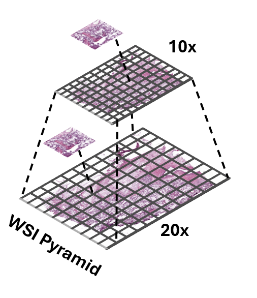
MethodCombine four expert-role prompts and reasoning-informed text embeddings with 10×/20× visual features using learned patch prototypes and cross-attention.
FindingUnder the 16-shot, five-fold protocol, the best configurations reach AUC 0.9604 ± 0.0088 on TCGA-RCC and 0.8770 ± 0.0195 on TCGA-NSCLC, outperforming 20 MIL baselines.
ImpactExpert-derived language and multi-scale visual evidence can support subtyping with few labelled slides; gains depend on the encoder and prompting configuration.
TME-Context
ConferenceUnder review
Conditioning pathology vision–language models on quantitative tumor-microenvironment measurements
Big ideaGive pathology vision–language MIL models explicit tumor-microenvironment context: quantitative TME measurements derived from the H&E slide itself.
TC-LRAn H&E TME atlas model produces OpenTME measurements; after scaling, a regularized logistic regressor predicts the subtype from TME features alone.
TC-FusionBlends the native VLM prediction with the TME prediction: (1 − α)·pnative + α·pLR.
TC-AdapterGroups TME features into 16 phenotype tokens that cross-attend to the frozen VLM’s patch features, yielding TME-conditioned queries for the aggregator. Works with ViLa-MIL, MGPATH, FOCUS, MUSE, DyKo and MSCPT.
INVEX
Label-free FM ranking
Label-free pathology foundation model ranking via invariance and expressiveness
Big ideaRank pathology foundation models intrinsically, from their embeddings alone: no labels, no fine-tuning.
InvarianceA patch rotated by 90°, 180° or 270° has the same morphology, so its embeddings should stay close.
ExpressivenessEffective rank of the embeddings checks that different tissues stay apart instead of collapsing together.
Scale22 pathology FMs, 16 public patch-level benchmarks, 8+ organs and more than 1.2M patches.
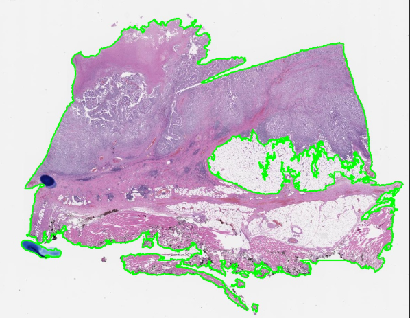
Whole-slide image processing
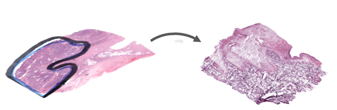
Tissue with pen marksAfter artifact filtering
TRIDENT segments tissue, then applies GrandQC to exclude artifacts from the tissue mask. The retained contours are saved as GeoJSON for patch selection.
MethodBenchmark 18 state-of-the-art vision and vision-language pathology encoders across 4,331 TCGA and CPTAC whole-slide images, evaluating similarity, representation alignment, and downstream transferability.
12
Patch Encoders
6
Slide Encoders
13
Downstream Tasks
4,331
Total Slides (TCGA & CPTAC)
47.5M+
Extracted Patches
3
Organs (Breast, Lung, Colon)
229
Property Tests
20x, 10x, 5x
Magnifications
Research questions
MOSAIC
Do independently trained pathology foundation models learn the same thing?
Central hypothesis: Independently trained pathology foundation models learn different coordinate systems over a shared underlying morphological manifold.
If that holds, representations should be alignable, semantic neighbourhoods should survive alignment, features should transfer between models, and a downstream classifier should be able to live inside one shared space.
Linear CKA
Do two encoders arrange the same patches the same way? Compare who sits near whom, ignoring rotation and scale.
Pseudocode
X = enc_a(patches) # n x d_xY = enc_b(patches) # n x d_yX = X - X.mean(0)Y = Y - Y.mean(0)K, L = X @ X.T, Y @ Y.T # n x nhsic = norm(X.T @ Y) ** 2den = norm(X.T @ X) * norm(Y.T @ Y)cka = hsic / den# cka(X @ Q, 3 * Y) == cka(X, Y)
Two representations
the same patches, in the same row order
feature widths may differ
Run the same patches through two encoders.
Each patch is one row in and the same row in .
Center the features
centering matrix: removes each feature's mean
Subtract each feature’s average.
Now only the shape of the cloud matters, not where it sits.
Sample-wise geometry
how patch relates to patch in encoder A
For every pair of patches, measure how alike each encoder thinks they are.
Each encoder gets its own “who resembles whom” table.
Linear CKA
Frobenius norm, the square root of the sum of squared entries
1 means the two geometries match
Lay the two tables on top of each other and check agreement.
Normalize: 0 = unrelated, 1 = same geometry.
Invariances
notinvariant to an arbitrary invertible linear map
Rotating or uniformly rescaling an encoder changes nothing.
CKA compares structure, not the axes each model happened to pick.
Kernel CKA
Linear CKA with local, curved similarity: two encoders can match even if one bends the other’s geometry.
Pseudocode
X, Y = enc_a(patches), enc_b(patches)defrbf(A, s): D = cdist(A, A) ** 2 return exp(-D / (2 * s * s))K, L = rbf(X, s_x), rbf(Y, s_y)H = eye(n) - ones((n, n)) / nKc, Lc = H @ K @ H, H @ L @ Hnum = (Kc * Lc).sum()cka = num / (norm(Kc) * norm(Lc))
Nonlinear relationship
curveda straight-line comparison can miss this
Two encoders can bend the same structure differently.
A straight-line comparison may miss that they agree.
RBF kernel
bandwidth; often set from the median pairwise distance
Score each pair of patches by closeness: near ≈ 1, far ≈ 0.
σ sets how far “near” reaches.
Kernel matrices
one entry per pair of patches
Build one closeness table per encoder.
Neighbours along a curve light up a band near the diagonal.
Center the kernels
removes the mean similarity of every row and column
Subtract the average closeness of every row and column.
What is left: how much more or less alike a pair is than usual.
Kernel CKA
gives back linear CKA
Compare the two centered tables as in linear CKA.
Bent but matching geometries still score high.
SVCCA
Keep only each encoder’s dominant directions, then ask how well those directions can be lined up.
Pseudocode
X, Y = enc_a(p), enc_b(p)defkeep99(A): U, s, _ = svd(A - A.mean(0)) r = cumsum(s**2) / sum(s**2) k = searchsorted(r, .99) + 1 return U[:, :k] * s[:k]Xr, Yr = keep99(X), keep99(Y)rho = cca(Xr, Yr) # canonical correlations# rho[0] >= rho[1] >= ... >= rho[K-1]svcca = rho.mean()
Two representations
the two encoders can have different widths
Two encoders, same patches, different numbers of features.
Do they capture the same information?
SVD: keep dominant directions
components kept per encoder
drops low-variance, noisy directions
Keep only the directions carrying 99% of each encoder’s variation.
This drops noisy, nearly empty directions.
CCA: first pair
weights: one linear combination of features per encoder
Find one mix of A’s features and one of B’s that move together most.
Their correlation ρ₁ says how well that best pair lines up.
More pairs
correlations come out in decreasing order
Find the next-best pair, unrelated to the ones already found.
Repeat: correlations come out from strongest to weakest.
SVCCA score
canonical pairs, at most min(k_a, k_b)
Average the correlations into one score.
High = the encoders share their dominant directions.
PWCCA
SVCCA where each matched direction counts by how much of the representation it actually carries.
Pseudocode
rho, A, B = cca(X, Y)H = X @ A # canonical variates# SVCCA would use rho.mean()alpha = abs(H.T @ X).sum(1)alpha = alpha / alpha.sum()# wide bar: explains much of Xpwcca = (alpha * rho).sum()
Start from CCA
CCA weights, as in SVCCA
Start from the CCA directions and their correlations, as in SVCCA.
The problem with a plain mean
noiseweak, low-ρ directions count as much as strong ones
A plain average treats every direction the same.
Weak, noisy directions drag the score down unfairly.
Projection weights
feature of : one column
share of that direction accounts for
Ask how much of A’s features each direction actually explains.
Directions that carry more of the representation weigh more.
Weighted correlations
areabar width × height = contribution to the score
Each bar’s width is now its importance.
Important directions dominate; noise barely shows.
PWCCA score
asymmetricweights come from ; one can average both directions
The score is the importance-weighted average correlation.
Weights come from one side, so A→B and B→A can differ.
Procrustes similarity
Can one rigid rotation lay one point cloud on top of the other? The tighter the fit, the more similar.
Pseudocode
X, Y = enc_a(p), enc_b(p)X = X - X.mean(0); X /= norm(X)Y = Y - Y.mean(0); Y /= norm(Y)U, s, Vt = svd(X.T @ Y)R = U @ Vt # orthogonalproc = s.sum() # nuclear normdist = 2 - 2 * proc # ||XR - Y||^2
Paired point clouds
pairsrow of and row of are the same patch
zero-pad the narrower one
Same patches, but the two clouds are rotated, scaled and shifted.
Center and normalise
removes global scale
Move both clouds to the origin and give them the same size.
Only the difference in orientation remains.
Best rotation
one rotation or reflection for the whole space
Find the single rotation that lays A’s cloud onto B’s.
Turning or mirroring only: no stretching.
Procrustes similarity
nuclear norm: the sum of singular values
Measure the overlap after that best rotation.
High = same shape up to a rigid turn.
A distance in disguise
stricterCCA may reweight each direction; Procrustes may not
CCA may stretch each direction to force a match; Procrustes may not.
So Procrustes is the stricter test of “same shape”.
Cosine RSA
Each encoder judges how alike every pair of patches is; RSA asks whether the two sets of judgements agree.
Pseudocode
X, Y = enc_a(p), enc_b(p)Xn = X / norm(X, axis=1, keepdims=True)Yn = Y / norm(Y, axis=1, keepdims=True)Cx, Cy = Xn @ Xn.T, Yn @ Yn.Tiu = triu_indices(n, k=1)vx, vy = Cx[iu], Cy[iu]rsa = spearmanr(vx, vy)[0] # or pearsonr
Embeddings as directions
patcheach one is a direction from the origin
Treat each patch’s embedding as an arrow from the origin.
Cosine similarity
angle between two embeddings; length is ignored
Compare two patches by the angle between their arrows.
Length is ignored; only direction counts.
Similarity matrices
RSMrepresentational similarity matrix
Fill a table with that similarity for every pair of patches.
One table per encoder.
Keep the upper triangle
the diagonal is always 1 and the matrix is symmetric
Keep each pair once and line the pairs up as a list.
Both encoders’ lists use the same pair order.
Correlate the patterns
Pearson, or Spearman to compare rankings only
Correlate the two lists.
High = the encoders agree on which patches are alike.
Distance correlation
Do distances in one encoder predict distances in the other? Catches any dependence, linear or not.
Pseudocode
A = cdist(X, X) # n x nB = cdist(Y, Y)defdc(D): r, c = D.mean(1, keepdims=True), D.mean(0) return D - r - c + D.mean()Ah, Bh = dc(A), dc(B)dcov2 = (Ah * Bh).mean()dvar = sqrt((Ah**2).mean() * (Bh**2).mean())dcor = sqrt(dcov2 / dvar)
Pairwise distances
distanceswork for any widths d_x and d_y
Measure the distance between every pair of patches, in each encoder.
Distance matrices
one entry per pair of patches
Collect them into two distance tables.
Double centering
mean of row ; ā.. is the grand mean
Remove each row’s and column’s average distance.
This keeps how unusually close or far each pair is.
Distance covariance
double-centered the same way
Multiply the two tables entry by entry and average.
Large when both encoders flag the same pairs as unusual.
Distance correlation
Normalize to 0–1; it is 0 only if the two are independent.
Unlike ordinary correlation, it also catches curved links.
Metrics side by side
The seven similarity metrics: each ignores some changes and catches others. That is why they can disagree on the same pair of encoders.
Score unchanged by
Sees nonlinear relations
Watch out
Metric · what it compares
Rotation
Scale
Shift
Any linear map
Linear CKAWho sits near whom, as one Gram matrix
Dominated by the largest-variance directions
Kernel CKAThe same, with a local RBF closeness
The bandwidth σ changes the answer
SVCCAThe best-matched directions after SVD
Depends on how many directions you keep
PWCCACCA directions, weighted by importance
One-sided by design; averaged both ways
ProcrustesOverlap after one best rotation
Rigid only: a stretched copy scores lower
Cosine RSAAgreement of pairwise-similarity rankings
Ignores embedding length entirely
Distance correlationWhether distances co-vary, in any way
Memory grows with n², from n × n distance tables
The score ignores this change The score is sensitive to it
GCCA
Find one shared coordinate system that every encoder can be linearly mapped into.
Pseudocode
Xs = [enc(p) for enc in encoders]C = lambda X: inv(X.T @ X + eps * I)Ps = [X @ C(X) @ X.T for X in Xs]vals, vecs = eigh(sum(Ps))G = vecs[:, -k:] # n x kWs = [C(X) @ X.T @ G for X in Xs]Zs = [X @ W for X, W in zip(Xs, Ws)]# every Z_m is close to G
Many encoders
encoders; shared patches
Several encoders, the same patches, each with its own axes.
What each view can express
projects onto what view can express
small ridge for stability
Work out which patterns each encoder can express.
Add them up: patterns every encoder can express stand out.
The shared space
shared dimensions
The strongest shared patterns become the common space .
Map every view
a linear map per encoder
Give each encoder its own linear map into .
After mapping, all encoders’ points land on the same spots.
Objective
MAXVARthis formulation of GCCA
Everyone connects to one shared hub.
A new patch from any encoder gets the same coordinates.
MCCA
Find one projection per encoder so that all encoders agree with each other, pair by pair.
Pseudocode
Xs = [enc(p) for enc in encoders]C = cov(hstack(Xs)) # blocks C_mlD = block_diag(C_11, ..., C_MM)# z_m = X_m @ w_mvals, W = eigh(C, D) # generalizedWs = split(W[:, -K:], dims)Zs = [X @ Wm for X, Wm in zip(Xs, Ws)]
Many encoders
encoders, same patches
Several encoders, the same patches.
Every pair
all pairsevery encoder is compared with every other
No shared hub: compare every pair of encoders directly.
One projection per view
weights: one linear combination per encoder
Squash each encoder’s features into one number per patch.
Sum of pairwise correlations
cross-covariance between views and
SUMCORthis sum-of-correlations criterion
Choose the squashing weights so every pair agrees as much as possible.
All pairwise scatter plots tighten at once.
More components
solvea generalized eigenproblem on the block covariance
GCCA aligns everyone to a shared target; MCCA aligns them to each other.
Both are linear.
Generalized Procrustes
Rotate every encoder onto a running average shape until they all settle on one consensus.
Pseudocode
Xs = [center_unit(X) for X in Xs]mean = Xs[0]for it in range(T): Rs = [procrustes(X, mean) for X in Xs] Al = [X @ R for X, R in zip(Xs, Rs)] mean = sum(Al) / M mean /= norm(mean)aligned = Al # one rotation per view
Center and normalise
zero-pad to a common width
Center each encoder’s cloud and give it unit size.
Pick a reference
referenceany view works; the result is the same up to one rotation
Take one encoder as the first guess of the average shape.
Rotate onto the mean
rotation or reflection only: shapes are kept
Rotate every encoder onto that average shape.
Rotation only: shapes are never stretched.
Update the mean, repeat
repeatuntil the mean stops moving
Average the rotated clouds into a new mean, then repeat.
The misfit shrinks until the mean stops moving.
Objective
the consensus shape all encoders share
Result: one consensus shape, plus one rotation per encoder.
Joint PCA
Put all encoders’ features side by side and keep the few directions that explain them together.
Pseudocode
Xs = [enc(p) for enc in encoders]Xs = [X - X.mean(0) for X in Xs]Xs = [X / norm(X) for X in Xs]Xc = hstack(Xs)U, s, Vt = svd(Xc, full_matrices=0)Z = U[:, :k] * s[:k] # n x kVs = split(Vt[:k].T, cumsum(dims)[:-1])
Views
widths may differ
Each encoder gives a feature table of a different width.
Scale and concatenate
a common scaling so no view dominates
centered view
Scale each table so none dominates, then glue them side by side.
PCA on the joint matrix
joint principal directions
Run PCA on the glued table.
Keep the few directions that explain the most combined variation.
Shared coordinates
size of the shared subspace
Those directions give every patch a short shared coordinate.
Each encoder owns a slice of the directions.
Per-view loadings
rows of that belong to view
A patch’s coordinate is the sum of every encoder’s contribution.
No agreement goal: it chases variance, so scaling matters.
Shared autoencoder
Learn nonlinear maps into one small code from which every encoder’s features can be rebuilt.
Pseudocode
xs = [enc(p) for enc in encoders]zs = [E[m](xs[m]) for m in range(M)]align = sum(mse(zs[m], zs[l]) for m < l)rec = sum(mse(D[l](z), xs[l]) for z in zs for l in range(M))loss = rec + lam * alignloss.backward(); opt.step()
Inputs
widths may differ
Each encoder describes the same patch with a different-length vector.
Encode
small MLP per encoder
bottleneck size
A small neural network per encoder squeezes it into a short code.
One shared bottleneck
same patchits codes should coincide
Train the codes from all encoders to agree for the same patch.
Decode every view
decoder for view
From that single code, rebuild every encoder’s features.
Training loss
weight on agreement; one common recipe, details vary
Training cuts rebuild error and disagreement together.
Being nonlinear, it can line up curved structure.
Aligners side by side
The five alignment methods all build one shared space from many encoders. They differ in what they treat as the reference and how freely each encoder may move.
Method
Shared reference
Map for each encoder
Objective
Watch out
GCCA
One central space G
A linear map W per encoder
Every encoder agrees with G
Linear only
MCCA
None: encoders meet pairwise
A linear projection per encoder
Sum of all pairwise correlations
Pairs grow fast as encoders are added
Generalized Procrustes
A consensus mean shape
A rotation per encoder
Least-squares fit to the mean
Cannot stretch; pad to one width
Joint PCA
Top joint principal axes
PCA loadings, split by encoder
Most joint variance
Variance, not agreement; scaling matters
Shared autoencoder
One small shared code
An MLP encoder and decoder per encoder
Rebuild every view; codes agree
Needs training and tuning
Icons, with example encoders: UNI-v2 CONCH Virchow2
Cross-model transfer
Encode a patch with one model and decode it as another: can a model built on B use A’s features unchanged?
Why a queue?SimCLR’s negatives are limited to the batch. A queue of past keys holds far more.
Pseudocode
for x in loader: x_q, x_k = aug(x), aug(x)# f_k initialized from f_q q = f_q(x_q) # N x C k = f_k(x_k).detach()# queue: C x K keys, past batches l_pos = (q * k).sum(1, True) # N x 1 l_neg = q @ queue # N x K logits = cat([l_pos, l_neg], 1) labels = zeros(N) # positive at 0 loss = CE(logits / t, labels) loss.backward(); opt.step() # f_q f_k = m * f_k + (1 - m) * f_qenqueue(queue, k); dequeue(queue)# v2: MLP head, blur, cosine lr, t=0.2
Query and key views
crop, color jitter, flip, grayscale (v1)
Two random views of one patch; training pulls them together.
Two encoders
query encoder, trained by backpropagation
key encoder: no gradients, initialized from f_q
The key encoder is a slow, gradient-free copy of the query encoder.
Normalized embeddings
128ResNet-50, then fc to 128-d, ℓ2-normalized
detached; key batch shuffled across GPUs (shuffling BN)
Each view becomes a unit vector: or .
Dictionary as a queue
negatives come from the queue, decoupled from the batch size (256)
The dictionary of negatives can be far bigger than the batch.
InfoNCE over keys
the key of the same image, at index 0
0.07 in v1
Train to find its own key among .
Momentum update
momentum coefficient, 0.999
Slow drift keeps old and new keys in the queue comparable.
Update the queue
queuekeys from recent batches by a slowly changing encoder
This batch’s keys join; the oldest batch leaves.
MoCo v2 changes
Component
MoCo v1
MoCo v2
Projection head
Single linear layer
2-layer MLP with ReLU
Data augmentation
Standard augmentation
Stronger augmentation, including Gaussian blur
Learning-rate schedule
Step decay
Cosine decay
Temperature
0.07
0.2
Barlow Twins
H&E patch (unlabeled)
Two random augmentations(as in BYOL, incl. solarization)
View
random crop, then augment
View
random crop, then augment
Twin AEncoder ResNet-50Projector, 3 layers
Twin B, same weightsEncoder ResNet-50Projector, 3 layers
Shared weights
8,192-d embedding
8,192-d embedding
Cross-correlation of the two embeddingscomputed over the batch; 8 of the 8,192 dimensions shown
batch × , each column standardized
,
Diagonal → 1: each dimension is invariant to the augmentations
Off-diagonal → 0: dimensions carry non-redundant information
Training drives toward the identity
No negatives, predictor, stop-gradient or momentum encoder
Downstream: keep and its 2,048-d output ; drop
Pseudocode
# x: N unlabeled H&E patchesfor x in loader: y_a, y_b = augment(x), augment(x) h_a, h_b = f(y_a), f(y_b) # shared z_a, z_b = g(h_a), g(h_b) # N x D z_a = (z_a - z_a.mean(0)) / z_a.std(0) z_b = (z_b - z_b.mean(0)) / z_b.std(0) c = z_a.T @ z_b / N # D x D on = ((diag(c) - 1) ** 2).sum() off = (off_diagonal(c) ** 2).sum() loss = on + lambd * off loss.backward(); opt.step()# after training: keep f, use h
Two augmented views
crop, flip, color jitter, grayscale, blur, solarization
independent draws; blur and solarization odds differ per view
One encoder, shared weights
encoder (ResNet-50), the same weights for both views
2,048-d representation kept for downstream tasks
A wide projector
projector: 3 linear layers of 8,192 units
BN, ReLUafter the first two layers
Standardize each dimension over the batch
mean and standard deviation of dimension over the batch
a sample in the batch (2,048 in the paper)
Cross-correlation between the views
, entries between −1 and 1
embedding dimensions, not samples
Barlow Twins loss
5 × 10⁻³, weights the redundancy term
invariance: each dimension agrees across views
redundancy reduction: dimensions decorrelate
Target
identity matrix
nonegatives, predictor, stop-gradient or momentum encoder
VICReg
H&E patch (unlabeled)
Two random augmentations(as in BYOL, incl. solarization)
View
random crop, then augment
View
random crop, then augment
BranchEncoder ResNet-50Expander, 3 layers
Branch′Encoder ResNet-50Expander, 3 layers
Shared weights(or not: may differ)
8,192-d, not normalized
8,192-d, not normalized
Invariance
Pull the two embeddings together (MSE)
VarianceKeep each dimension’s std above , per branchCovariance
Decorrelate dimensions within each branch
No negatives, stop-gradient, predictor or embedding normalization
Downstream: keep and its 2,048-d output ; drop
Pseudocode
for x in loader: x_a, x_b = augment(x), augment(x) y_a, y_b = f(x_a), f(x_b) z_a, z_b = h(y_a), h(y_b) # N x D sim = mse_loss(z_a, z_b); v = c = 0for z in (z_a, z_b): # each branch std = sqrt(z.var(0) + 1e-4) v += relu(1 - std).mean()for z in (z_a, z_b): C = cov(z) # D x D c += off_diag(C).pow(2).sum() / D loss = 25 * sim + 25 * v + 1 * c loss.backward(); opt.step()
Two augmented views
the image; and are its two views
crop, flip, color jitter, grayscale, blur, solarization
An encoder per branch
encoder (ResNet-50); its 2,048-d output is kept
usually equal to , but the branches may differ
Expander
expander: 3 layers of 8,192 units, discarded after training
a batch of embeddings, not normalized
Invariance
batch size (2,048 in the paper)
the only term that links the two branches
Invariance: Pulls two augmented views of the same image closer together.
Variance (hinge on the std)
target standard deviation, 1
10⁻⁴, keeps the square root stable
dimension across the batch, per branch
Variance: Prevents different images from all being mapped to the same representation.
Covariance, within each branch
covariance within one branch
vs. BarlowBarlow Twins correlates the two branches
Covariance: Encourages different embedding dimensions to carry nonredundant information.
Total loss
ImageNet defaults
nonegatives, stop-gradient, predictor or normalization
Invariance: Pulls two augmented views of the same image closer together.
Variance: Prevents different images from all being mapped to the same representation.
Covariance: Encourages different embedding dimensions to carry nonredundant information.
DINO
H&E patch (unlabeled)
Multi-crop augmentation(crop, color jitter, blur, …)
Student views (global + local crops)
2 global crops (high resolution)
•••
Several local crops (low resolution)
Global crops only(the student’s 2 global crops)
Teacher views (global only)
2 global crops (high resolution)
Student NetworkBackboneVision TransformerProjection head
Teacher NetworkBackboneVision TransformerProjection head
Cross-entropy between teacher and student output distributions from different views
Cross-entropy
EMA update
Pseudocode
# x: unlabeled H&E patchfor x in wsi_patches: crops = multi_crop(x) v_s = crops # 2 global + n local v_t = crops[:2] # same globals s = student(v_s)# teacher: stop gradientwith no_grad(): t = teacher(v_t) p_s = softmax(s / tau_s)# center, then sharpen p_t = softmax((t - c) / tau_t)# teacher global i vs student view j loss = mean(H(p_t[i], p_s[j])for i in (0, 1)for j in views if j != i) loss.backward() optimizer.step() # student teacher = ema(teacher, student) c = ema(c, t.mean(0))
Multi-crop views
all views of patch
2 global crops, 224 px
local crops, 96 px
number of local crops
Teacher views
the same 2 global crops
all views the student sees
Stop gradient
teacher weights, never trained by the loss
DINO loss
Student softmax
student logit for one view
output dimensions, 65,536 in DINO
student temperature, 0.1
Centered, sharpened teacher softmax
teacher logit
center, a running mean of
teacher temperature, warmed up from 0.04 to 0.07, below τₛ
Cross-entropy across views
cross-entropy
a teacher global crop; any other student view
EMA updates
student and teacher weights
momentum, 0.996 rising to 1
center momentum, 0.9 in the official code
batch mean of teacher outputs
MAE
H&E patch (unlabeled)
196 patches of 16 × 16 px
75% masked at random
25% visible
EncoderViT, visible patches only
Encoded tokens + shared mask token, with positions
Decoderlightweight
Masked patches predicted
Loss on masked patches onlymean squared error, per-patch normalized pixelspredictionvs.target
After pretraining, drop the decoder and run the encoder on all patches
Pseudocode
# x: N unlabeled H&E patchesfor x in loader: p = patchify(x) # B x 196 x 768 keep, mask = random_masking(0.75) z = encoder(p[keep] + pos[keep]) t = cat([z, m.repeat(n_masked)]) t = unshuffle(t) + pos p_hat = decoder(t)# p_hat: pixels for all 196 patches y = (p - p.mean(-1)) / p.std(-1) err = ((p_hat - y) ** 2).mean(-1) loss = err[mask].mean() loss.backward(); opt.step()# after: keep encoder, drop decoder
Patchify
one 16 × 16 px patch (7 × 7 of 196 shown)
Random masking
masked patches, sampled uniformly at random
Encoder on visible patches only
ViT encoder (ViT-B/16, L/16, H/14)
positional embedding of patch
25%of tokens enter the encoder, so pretraining is cheaper
Mask tokens join the sequence
one shared, learned mask token
Lightweight decoder
decoder: 8 blocks, 512-d, about 9% of ViT-L’s FLOPs per token
Reconstructed pixels
768= 16 × 16 × 3 pixel values per patch
Loss on masked patches
mean and std of patch i’s own pixels
the loss is computed on masked patches only
Downstream
discarded after pretraining
aug.random crop and flip only
I-JEPA
H&E patch (unlabeled)
4 target blocks, 15–20% each
Context: a large block minus the targets
Context encoderViT, context only
context representations
Predictornarrow ViT, per block
Predicted
EMA update
L2 loss on representations
averaged over the 4 target blocks
Target encoderEMA copy
masked after encoding
Targets
No hand-crafted augmentations: masking only
Pseudocode
# x: N unlabeled H&E patchesfor x in loader: blocks = sample_targets(4) # 15-20% ctx = sample_context() # 85-100% ctx = ctx - union(blocks) s_x = ctx_enc(x, keep=ctx)with no_grad(): s_y = tgt_enc(x) # full image loss = 0for b in blocks: pred = predictor(s_x, pos=b) loss += l2(pred, s_y[b]) loss = loss / len(blocks) loss.backward(); opt.step() tgt_enc = ema(tgt_enc, ctx_enc)
Target blocks
patch indices of target block ; blocks may overlap
size15–20% of the image each, aspect ratio 0.75–1.5
Context block
one block covering 85–100% of the image, square
patches inside any target block are removed
Context encoder
context encoder (ViT), sees only the context patches
Target encoder, masked after encoding
target encoder, sees the full image
targets are masked after encoding, not before
Predictor, once per block
narrow ViT predictor (384-d), run once per block
shared mask token plus the position of target patch
Loss in representation space
distance in representation space, not pixels
EMA target encoder
momentum, 0.996 rising linearly to 1
used downstream, average-pooled; no [CLS] token
iBOT
H&E patch (unlabeled)
Multi-crop + block masking(masks on the 2 global crops)
Student views (masked global + local crops)
2 global crops, 224 px (patches masked)
•••
Local crops, 96 px (no masks)
Global crops only(same 2 crops, no masks)
Teacher views (global only)
2 global crops, 224 px (unmasked)
Student NetworkBackboneViT, patch 16CLSpatchesShared head
Teacher NetworkBackboneViT, patch 16CLSpatchesShared head
Colored dots mark a method that also belongs to another family
Methods that combine families
Self-distillation
Clustering and prototypes
Masked image modeling
Contrastive
DINO ’21
MAE ’21
MoCo ’19
SimCLR ’20
iBOT ’21
I-JEPA ’23
DINOv2 ’23
DINOv2 combines three
EMA teacher from self-distillation
iBOT masking from masked image modeling
Sinkhorn-Knopp centering from clustering
In pathology
DINOv2
UNI, Virchow, Prov-GigaPath, H-optimus-0
iBOT
Phikon
MoCo v3-based
CTransPath
MAE
Campanella et al.
DINOv2 for pathology
1 · Augmentationcrop-and-resize → ECT
2 · Diversity regularizerKoLeo → KDE
DINOv2: crop, then resize
resize
Cells enlarged and stretched32% of the area becomes the whole view
ECT: crop from a larger region
Cells keep their sizecontext comes from real tissue, ±10% scale
Slides are scanned at fixed magnifications, so object scale barely varies; resizing adds distortion without much benefit.
Near-duplicate tilestissue repeats across slides and patients, so often
KDE stays boundedthe kernel is bounded, so gradients stay finite
Everything else is unchanged
Student + EMA teachermulti-crop views
DINO + iBOT lossesclass token and masked patches
Sinkhorn-Knoppcentering of the teacher
Only two swapscrop-and-resize→ECTKoLeo→KDE
Used in Virchow2 and Virchow2G (3.1M WSIs, 5×–40×) and by Kaiko, which swaps KoLeo for KDE. The rest of DINOv2 stays the same.
Pseudocode
# DINOv2 loop; two swaps for tissuefor tiles in loader:# before: RandomResizedCrop(224,# scale=(0.32, 1)) on a 224 tile src = read_region(wsi, 392) v = ect_crop(src, 224) # ~1x# before: KoLeo, -log(nn_dist)# blows up when tiles repeat sim = z @ z.T # z: l2-normed sim.fill_diagonal_(-inf) reg = logsumexp(5 * sim, 1).mean() loss = l_dino + l_ibot + 0.05 * reg loss.backward(); opt.step()
Same DINOv2 loss; two parts swapped
the crop augmentation: what changes first
the diversity regularizer: what changes second
Crop-and-resize (DINOv2)
fraction of the tile’s area kept (DINOv2 global crops)
local, resized to 96 px
Extended-context translation
a 392 × 392 px source region read from the slide
local98 px crops, same logic, fixed aspect ratio
KoLeo (DINOv2)
-normalized class token of image
its gradient for nearest distance d; explodes as near-duplicate tiles get close
KDE regularizer
kernel concentration (how local the push is)
penalty stays at most κ and the gradient fades to 0: no blow-up
Everything else is unchanged
samestudent, EMA teacher, DINO and iBOT losses, Sinkhorn-Knopp
Where it is used
Virchow23.1M WSIs, mixed 5×–40× magnification
Kaikoalso replaces KoLeo with KDE
Slide foundation models
Patch encoderfrozen, e.g. UNI
tile features
Slide encoderpretrained: the aggregator
Slide embeddingone vector per slide
Patch FMs pretrain the tile encoder. Slide FMs also pretrain the aggregator, so one embedding per slide supports linear probing, retrieval and, with language, zero-shot use, without training a new MIL model per task.
Self-supervised on tile features
No labels: the slide’s own tile embeddings are the signal
HIPT ’22
Hierarchical ViT; DINO on 256 px patches, then 4K regions10,678 WSIs
Prov-GigaPath ’24
LongNet (dilated attention); MAE on tile embeddings171,189 WSIs
TITAN-V ’24
ViT on feature grids with 2D ALiBi; iBOT335,645 WSIs
COBRA ’24
Mamba-2 + gated attention; contrastive across patch FMs
Slide-level augmentation works on coordinates: crop 87.5% of the tile grid, shift it at random, flip horizontally with .
Downstream: a shallow attention-MIL head on the slide encoder. Vision–language variant: contrastive with PubMedBERT on 17,383 slide–report pairs.
Pseudocode
# slide: 256 px tiles + (x, y), 20xfor tiles, xy in slides:with no_grad(): h = tile_enc(tiles) # N x 1536 z = proj(h) + pos2d(xy // 256) z = cat([cls, z])# LongNet: dilated attention over z m = random_mask(N) o = longnet(z[:, ~m]) h_hat = decoder(o, m) loss = mse(h_hat[m], h[m])# aug: crop 87.5% of grid, shift, flip# downstream: ABMIL head on longnet(z)
Tiles with coordinates
256 × 256 px tile at 20× (0.5 µm/px)
tile position on the slide
Tile encoder (stage 1)
ViT-g/14 trained with DINOv2 on 1.3B tiles
frozenduring slide-level pretraining
Sequence with 2D positions
fixed sine–cosine table on a 1,000 × 1,000 grid
learned token; its output is the slide embedding
Dilated attention (LongNet)
segment lengths 1,024 … 1,048,576 tiles
dilation: keep every r-th token in a segment
costlinear in instead of quadratic
Slide-level masked autoencoder (stage 2)
masked tile positions
reconstruction from the visible tiles
Slide-level augmentation
crop87.5% of the tile grid, randomly shifted
flipcoordinates flipped horizontally,
Downstream use
shallow attention-MIL head, fine-tuned per task
VLCLIP-style with PubMedBERT, 17,383 slide–report pairs
· contrastive + 2.0 · captioning. Trained on specimens (several WSIs, one report): 587,196 WSIs, 195,344 reports. Inference usually runs on one slide.
Pseudocode
# a specimen: several WSIs, one reportfor wsis, report in specimens: h = virchow(tiles(wsis)) # N x 2560 lat = perceiver(L, h) # 513 x 1280 e_s, mem = lat[0], lat[1:] t = biogpt_uni(report + [CLS]) l_con = clip_loss(e_s, t[-1]) z = biogpt_multi(t[:-1], cross=mem) l_cap = CE(z[:-1], report[1:]) loss = 1.0 * l_con + 2.0 * l_cap loss.backward(); opt.step()
Specimen-level pairs
587,196 WSIs in 195,344 specimens
clinical report, condensed by GPT-4 (5 rewrites)
Virchow tile embeddings
VirchowViT-H/14, DINOv2; 224 px tiles at 20×
class token and mean patch token, 1,280-d each
Perceiver aggregator
cross-attention; latent self-attention
sharedweights shared across blocks
Two outputs
1 latent: the slide embedding
512 latents: memory for the decoder
Contrastive loss
unimodal layers, causal, text only
projboth embeddings → 5,120-d; learned temperature
Report generation loss
+ new cross-attention to
frozenBioGPT weights except word embeddings
CoCa-style objective
zero-shotclassify by comparing with text prompts
reportsfree-text report generation
CHIEF
256 px tiles at 10×
Tile encoderCTransPath
+ site
“This is a histopathological image of the [site].”
Text encoderCLIP, pretrained
2 FC layers
Attention aggregationclass-specific scoresdetails
Slide embeddingattention-pooled
Instance branchtiles ranked by attention; extremes become pseudo-labels
1
1
0
0
WSI-level contrastive branchmemory bank per cancer type (types shown are examples)
Pretraining
60,530 WSIs, 19 anatomic sites, 14 cohorts
Weak labels at the WSI level only
Tasks: cancer detection, tumor origin, genomic profiles, survival
Pseudocode
# slide, its site, its WSI-level labelfor tiles, site, y in slides: h = ctranspath(tiles) # 10x, 256 px T = clip_text(prompt(site)) h = h + mlp(T) a = attention(h) # per class e = (a[:, :, None] * h).sum(1) l_wsi = CE(cls(e), y)# top-attended tiles -> 1, bottom -> 0 l_inst = CE(inst(h[ext]), pseudo) l_con = bank_contrast(e, y, banks)# weighting not given in the paper loss = l_wsi + l_inst + l_con
Tiles
tile at 1.0 µm/px, background removed (Otsu)
Unsupervised tile encoder
Swin-based encoder, SSL on ~15M tiles
Anatomic-site text fusion
“This is a histopathological image of the [site].”
two fully connected layers
Attention aggregation
learned attention of tile for class
slide representation used for class
Instance branch
pseudo-label for tile , from attention rank
WSI-level contrastive branch
memory bank of slide embeddings for cancer type
lossgiven in the paper’s supplement
Weakly supervised pretraining
60,530WSIs, 19 anatomic sites, 14 cohorts, ~44 TB
weakWSI-level labels only
TITAN
512 px patches at 20×
Patch encoderCONCH v1.5
feature grid, 768-d each
Views of one region2 global 14×14, 10 local 6×6
Slide encoderViT, 6 layers, 768-ddetails
2D ALiBibias falls off with distance
details
Stage 1 · TITAN-V
iBOT on feature grids: student vs. EMA teacher, masked features
One slide encoder serves linear probing, few-shot, zero-shot classification, slide and rare-cancer retrieval, slide–report retrieval and report generation.
Pseudocode
# WSI -> 512 px patches at 20xfor wsi in slides: F = conch15(patches) # grid, 768-d R = crop(F, 16, 16) # 8K px region g, l = views(R, 2 * [14], 10 * [6])# ALiBi: bias = -m * dist(p_i, p_j) loss = ibot(stu(g, l), tea(g))# -> TITAN-V# stage 2: ROI + synthetic captionloss = coca(titan(R), caption)# stage 3: WSI + reportloss = coca(titan(F), report)
Patches at 20×
512 × 512 px patch at 20×, position
Feature grid
patch encoder, frozen; 768-d features
Views of a region
region crop the encoder trains on
aug.flips and posterization in feature space
Slide encoder with 2D ALiBi
grid position of patch
per-head slope; train on 8K regions, run on whole slides
Stage 1: vision-only (iBOT)
TITAN-Vthe vision-only model after stage 1
Stage 2: ROI captions (CoCa)
stage 2423,122 ROIs with PathChat captions
pooler1 contrastive + 128 reconstruction queries
Stage 3: reports (CoCa)
stage 3182,862 WSIs with pathology reports
Mass-340K335,645 WSIs, 20 organs
MADELEINE
H&E
ER (IHC)
HER2 (IHC)
stains recolored for illustration
Patch encoderCONCH, all stains
Slide encoder4-head attention MILdetails
+ stain embeddinglearnable, 32-d
Global: InfoNCEH&E vs. each other stain, both directions
The H&E slide embedding should match the same case’s stain embedding and not other cases’.
Local: graph optimal transportmatch patches (nodes) and their relations (edges)
Only H&E is needed downstream: the encoder learned from IHC what to look for.
Pseudocode
# a case: H&E + other stainsfor he, stains in cases: h = conch(tiles(w)) # every stain e = mh_abmil(h + stain_emb) l = info_nce(e_he, e_s) # each s l += got(h_he, h_s) # each s# downstream: mh_abmil(h_HE) only
Multistain pairs
breast4,211 WSIs from 1,153 cases (ER, PR, HER2, Ki-67)
Each slide is matched to its own molecular profile within the batch.
Pretraining data
47,171 WSIs with molecular profiles
MGH, BWH, TCGA, GTEx
26,615 with RNA; 20,556 with DNA panels
Molecular prompting
Build one prototype per class by averaging molecular embeddings
Classify a slide by its nearest prototype, with no task-specific training
Pseudocode
# WSI + bulk RNA or DNA panelfor wsi, mol in pairs: h = proj(conch15(tiles(wsi))) e = gated_abmil(h, heads=2) g = scgpt(mol) if rna elsemlp(mol) loss = clip_loss(e, g) loss.backward(); opt.step()# prompting: nearest prototype
Patches
512 × 512 px patch at 20×
Patch features
ViT-L patch encoder, frozen
projection 768 → 1,024
Slide encoder: gated attention MIL
heads2; slide encoder has 11.3M parameters
1,024-d slide embedding
Molecular encoders
12 blocks, pretrained on 5.7M cancer cells
DNAmulti-hot over 239 genes, 4-layer MLP
Slide–molecular contrastive loss
47,171WSIs: MGH, BWH, TCGA, GTEx
pairs26,615 with RNA, 20,556 with DNA
Molecular prompting
prototype of class from molecular profiles
SEAL: paired spots and patches
Towards Spatial Transcriptomics-driven Pathology Foundation ModelsHemker, Song et al., Mahmood Lab, arXiv 2026Paper ↗Code ↗Hugging Face ↗
Pseudocode
for spot in visium_sample.spots: s = random.choice([0.25, 0.5, 1.0]) x = crop(wsi, spot.center, 224, mpp=s) c = spot.counts g = log1p(1e4 * c / c.sum())[hvg] g = (g + G[spot.nbrs].mean(0)) / 2 pairs.append((x, g)) # 723,250 pairs
Paired measurements
Visiumspatial transcriptomics: expression measured in 55 µm spots on a hexagonal grid
Image side
spot centroid
one magnification sampled per spot, per step
Gene side
highly variable genes (Seurat v3)
2,000genes in training
Spatial smoothing
up to 6 neighbours on the hexagonal lattice
Training set
723,250 pairs from 353 samples, 14 organs
split80/10/10 by patient, stratified by organ
SEAL: two encoders
Pseudocode
vit = load_fm("uni_v2") # any of 5vit.requires_grad_(False)add_lora(vit.blocks[-k:], r=8, alpha=8)e = mlp(g) # Linear-BN-ReLUmu, logvar = w_mu(e), w_var(e)z = mu + exp(logvar / 2) * randn_like(mu)for f in planar_flows: z = f(z)g_hat = decoder(z) # mirrored MLPassert z.shape[-1] == vit.embed_dim
A Foundation Model for Spatial ProteomicsShaban, Chang et al., Mahmood Lab, arXiv 2025Paper ↗Code ↗Hugging Face ↗
Pseudocode
X = load_multiplex(roi) # H x W x M# 30 sources, 8 platforms, 16 tissuestiles = tile(X, 256, overlap=0.5)tiles = [t for t in tiles iftissue_ok(t)]t = (t - mu[markers]) / sd[markers]sub = random.choice(subsets) # 23x = t[[dapi, *sample(panel, 2)]]
A multiplex image
tens of markers per section (up to ~50–60)
channelone antibody, one fluorescence image
SPM-47M sources
30sources: 56% public, 44% in-house
8fluorescence platforms, e.g. CODEX, MxIF, COMET, IBEX
Patches
px patches, 50% overlap
single-marker patches from 3.67M multiplex patches
Quality control
QCmarkers checked against vendor / Human Protein Atlas staining; tissue mask drops folds, blur, saturation
Per-marker normalisation
per-marker statistics over the whole corpus
Training sample
23tissue–technology subsets; pick one, then a patch
aug224 crops, flips, 90° rotations
KRONOS: a marker-aware ViT
Pseudocode
for j in markers: xb[j] = embed(x[j]) # sharedm = sincos(marker_ids, D) # fixedz = xb + m[:, None] + pos[None]z = vit_blocks(cat([cls, z.flatten(0, 1)]))img = z[0]marker = z[1:].view(M, N, D).mean(1)tokens = z[1:].view(M, N, D)
Tokenise each marker
16 × 16 px patch of marker
same weights for every marker
Marker identity
fixed, not learned: an unseen marker just takes an unused index
Add the codes
Visual embedding of spatial patch from protein marker
Marker identity code: which protein?
Spatial positional embedding: where in the tissue patch?
Final token given to the transformer
For the CD3 channel, KRONOS constructs:
One sequence
tokens: attention mixes locations and markers
ViT-S/16backbone
Three outputs
image-level output
GigaTIME: paired H&E and mIF
Multimodal AI generates virtual population for tumor microenvironment modelingMicrosoft Research, Providence and UW, CellPaper ↗Code ↗Hugging Face ↗
Pseudocode
he, mif = load(case) # H&E WSI, COMET mIFmif = valis_register(mif, he)A, B = stardist(he), stardist(mif.dapi)keep tiles if dice(A, B) >= 0.2Y = mif > thresholds # per channelpairs.append((he_tile, Y)) # 256 x 256
Same tissue, two stains
COMETsequential mIF platform; same tissue as the H&E slide
Registration
rigid + non-rigid warp found by VALIS
image dissimilarity
Quality filter
StarDist cells on H&E / on mIF DAPI; 0.2 set from 100 hand-labelled pairs
Per-pixel targets
CD8 intensity
1280100451101402026090805203
t = 50 example
binary map
0110011001100000
Training pairs
2321 proteins + 2 background channels
cells in the paired training data
GigaTIME: a UNet++ translator
Pseudocode
x = he_tile # 3 x 256 x 256X[i][0] = conv(down(X[i-1][0]))X[i][j] = conv(cat(X[i][:j], up(X[i+1][j-1])))# every node sees all earlier nodes in its rowY_hat = sigmoid(conv1x1(X[0][4])) # 23 mapsloss = bce(Y_hat, Y) + 1 - dice(Y_hat, Y)# 300 epochs, Adam 1e-3, batch 32
Encoder
encoder node at depth
downsampling
Nested decoders
upsampling from the node below
Dense skips
concatenation: dense skip connections across the row
Output head
2321 protein + 2 background channels
BCE + Dice
Diceoverlap per channel; helps sparse markers
Training
300epochs; Adam, lr 10⁻³, batch 32 (released recipe)


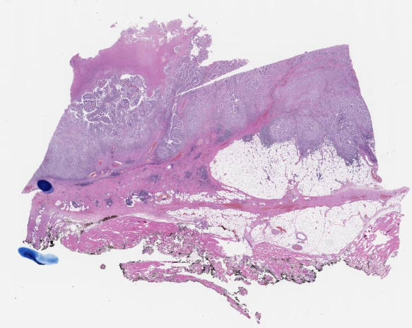 H&E slide
 Tissue contours