CLIP
- dense sheet of tumor cells
- irregular glands in pink stroma
- fibrous stroma, spindle nuclei
- gland lumen lined by tall cells
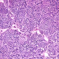
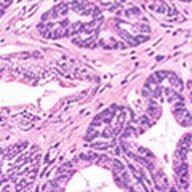
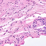
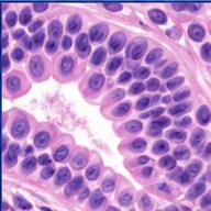
encoderResNet or ViT
Linear then -normalize
encoderTransformer
Linear -normalize
- Each cell:
- Diagonal: the true pairs (targets)
- Blue row: image 1 vs. all captions
- Orange column: caption 1 vs. all images
- Off-diagonal: mismatches
- Training lifts the diagonal, lowers the rest
imagecaption Each encoder starts in its own region Pairs line up; the regions stay apart A new image lands level with its class prompt
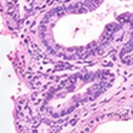
- an H&E image of tumor.0.05
- an H&E image of glands.0.91
- an H&E image of stroma.0.03
- an H&E image of fat.0.01
Pseudocode
# N (image, caption) pairs from the web
for imgs, texts in loader:
  i_e = l2norm(image_enc(imgs) @ W_i)
  t_e = l2norm(text_enc(texts) @ W_t)
  # both: N x d_e, unit length
  logits = exp(t) * i_e @ t_e.T  # N x N
  labels = arange(N)  # diagonal
  loss = (CE(logits, labels)
        + CE(logits.T, labels)) / 2
  loss.backward(); opt.step()
  t.clamp_(max=log(100))
# zero-shot, no training
T = l2norm(text_enc(prompts) @ W_t)
pred = argmax(i_e @ T.T)
A batch of image–caption pairs
- pairs per batch (32,768 in the paper)
- the web text that came with image ; ~400M pairs in total
Image embedding
- image encoder: ResNet or ViT
- a linear projection only, no MLP head
- random square crop is the only augmentation
Text embedding
- text Transformer; the [EOS] token is the feature
- a linear projection only
One shared space
- the joint dimension (512 for ViT-B/32)
- so a dot product is a cosine
similarity logits
- image scored against caption
- a learned log-scale
Symmetric cross-entropy
- rows: each image picks its caption
- columns: each caption picks its image
What training does
- mismatched pairs act as negatives
- gap images and captions keep separate regions
Learned temperature
- softmax temperature, learned as
- 100 cap that keeps training stable
Zero-shot classification
- embedding of “an H&E image of {label}.”
- any class you can name; no retraining
CoCa
Image
Caption , shifted right,
with [CLS] appended
encoderViT
256 image tokens
Generative pooler256 learned queries
decoder tokens
Contrastive pooler1 learned query
What each text position sees
Contrastive lossimage ↔ text over the batch, as in CLIP
cross-attention
irregularglandsinpinkstroma[EOS]Predicted next tokens
(targets: the caption)
Captioning losscross-entropy on each next token, given the image
Embeddingszero-shot classification and retrieval, as in CLIP
Decodercaptioning and VQA, as in an encoder–decoder
PathologyCONCH: CoCa on 1.17M histopathology image–caption pairs
Pseudocode
# x: images, y: caption token ids
for x, y in loader:
  v = vit(x)  # B x 256 x D
  v_gen = gen_pool(v)  # 256 q
  e_x = con_pool(v_gen)  # 1 q
  h = uni_dec(cat([y, cls]))
  e_y = h[:, -1]  # [CLS]
  l_con = clip_loss(e_x, e_y, sigma)
  z = multi_dec(h[:, :-1], v_gen)
  # next-token prediction
  l_cap = CE(z[:, :-1], y[:, 1:])
  loss = 1.0 * l_con + 2.0 * l_cap
  loss.backward()  # one pass, both
# embeddings: zero-shot, retrieval
# decoder: captions, VQA
An image–caption pair
- the image (288 × 288 in pretraining)
- alt-text, or JFT label names in a prompt
Image tokens
- ViT 18 × 18 patches, so 16 × 16 = 256 tokens
- width; encoder 86M (Base) to 1B (CoCa)
Attentional pooler
- generative pooler: 256 queries, fed to the decoder
- contrastive pooler: 1 query, on top of the first
Unimodal text decoder
- learnable token appended to the caption
- causal token sees only tokens up to ; no image
Contrastive loss
- normalized image and [CLS] embeddings
- learnable temperature, starting at 0.07
Multimodal text decoder
- split decoder layers cut in half: 12 + 12 (Base, Large)
- cross-attn text queries; image keys and values
Captioning loss
- the true earlier tokens (teacher forcing)
- softmax over the vocabulary at step
One objective
- λ_Con = 1, λ_Cap = 2 in the paper
- cost 1.18× contrastive-only; one forward–backward
Two ways to use it
- zero-shot classification and retrieval
- captioning and question answering